2 LEARNING PROBLEM
Notation
| symbol | meaning |
|---|---|
| a,b,c,N\dots | scalar number |
| \boldsymbol{w},\boldsymbol{v},\boldsymbol{x},\boldsymbol{y}\dots | column vector |
| \boldsymbol{X},\boldsymbol{Y}\dots | matrix |
| \mathbb{R} | set of real numbers |
| \mathbb{Z} | set of integer numbers |
| \mathbb{N} | set of natural numbers |
| \mathbb{R}^{D} | set of vectors |
| \mathcal{X},\mathcal{Y},\dots | set |
| \mathcal{A} | algorithm |
| operator | meaning |
|---|---|
| \boldsymbol{w}^{\intercal} | transpose |
| \boldsymbol{X}\boldsymbol{Y} | matrix multiplication |
| \boldsymbol{X}^{-1} | inverse |
Learning diagram
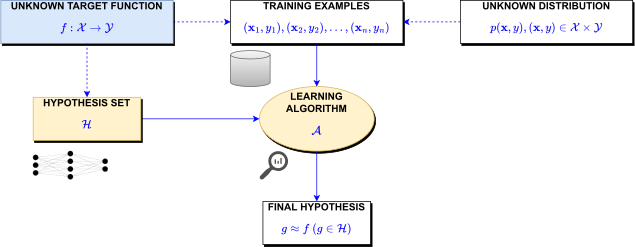
2.1 Learning Components
Credit Approval
Suppose that a bank receives thousands of credit card applications every day, and it wants to automate the process of evaluating them.
Applicant information
age 23 years gender male annual salary $30000 years in residence 1 year years in job 1 year current debt $15000 … … Approve credit?
Problem Statement
Formalization
Input: \boldsymbol{x} (customer application)
Output: y (good/bad customer? or \{1,-1\})
Data (\boldsymbol{x}_{1},y_{1}),(\boldsymbol{x}_{2},y_{2}),...(\boldsymbol{x}_{N},y_{N}) (historical records)
Target function: f:\mathcal{X}\to\mathcal{Y} (ideal credit approval formula)
Best approximate function g:\mathcal{X}\to\mathcal{Y} (formula to be used)
Inductive Bias
An unbiased learner can never generalize.
An inductive bias of a learner is the set of assumptions a learner uses to predict results given inputs it has not yet encountered.
- Consider: arbitrarily wiggly functions or random truth tables.
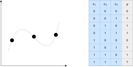
Inductive Learning Hypothesis Generalization is possible.
- If a machine performs well on most training data AND it is not too complex, it will probably do well on similar test data.
Components of Learning
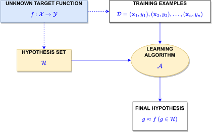
Learning Model
The two components are referred as the learning model
- The hypothesis set \mathcal{H} is a set of functions that is potentially similar to f \mathcal{H}=\{h_{\theta_{1}},h_{\theta_{2}},...\}
- The learning algorithm \mathcal{A} is a search algorithm which finds g\in\mathcal{H} such that g\overset{best}{\approx}f
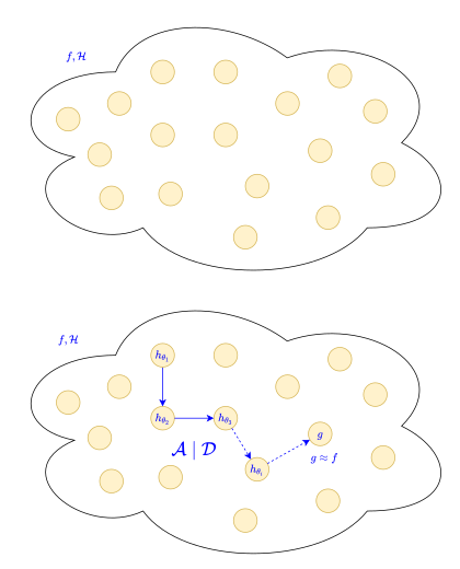
What is hypothesis set
Hypothesis set is a set of potential functions, models or solutions
Hypothesis set can be finite. For example
{guilty, not guilty}
{accept, reject}
{happy, sad}
{1,2,3,4,5,6}
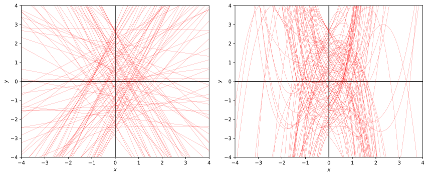
- Hypothesis set can be infinite. For example, sets of functions y={\color{red}\theta}_{0}+{\color{red}\theta}_{1}x and y={\color{red}\theta}_{0}+{\color{red}\theta}_{1}x+{\color{red}\theta}_{2}x^{2}+{\color{red}\theta}_{3}x^{3}
Parameter representations
Each element of hypothesis set often indexed by parameters or weights (\boldsymbol{{\color{red}\theta}} or {\color{red}\boldsymbol{w}})
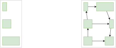
Two basic representations for parameters: factored, and structured
Factored: a paramater set consists of a vector of attribute values; values can be boolean, real-valued, or one of a fixed set of symbols.
Structured: a paramater set includes objects, each of which may have attributes of its own as well as relationships to other objects.
2.2 A Simple Learning Model
Hypothesis Set
A Simple Hypothesis Set
We starts with the simple model (the perceptron model)
For input \boldsymbol{x}=(x_{1},...,x_{d}) (attributes of a customer) \begin{align} \text{Approve credit if } & \sum_{i=1}^{d}{\color{red}w_{i}}x_{i}\geq{\color{red}threshold}\nonumber \\ \text{Deny credit if } & \sum_{i=1}{\color{red}w_{i}}x_{i}<{\color{red}threshold} \end{align}
This linear formula h\in\mathcal{H} can be written as \begin{equation} h(\boldsymbol{x})=h_{{\color{red}\boldsymbol{w},threshold}}(\boldsymbol{x})=\text{sign}\left(\left(\sum_{i=1}^{d}{\color{red}w}_{{\color{red}i}}x_{i}\right)-{\color{red}threshold}\right) \end{equation}
Set {\color{red}w_{0}}=-{\color{red}threshold} \begin{equation} h(x)=h_{{\color{red}\boldsymbol{w}}}(x)=\text{sign}\left(\left(\sum_{i=1}^{d}{\color{red}w}_{{\color{red}i}}x_{i}\right)+{\color{red}w_{0}}\right) \end{equation}
Introduce an artificial coordinate x_{0}=1 \begin{equation} h(x)=h_{{\color{red}\boldsymbol{w}}}(x)=\text{sign}\left(\sum_{i=0}^{d}{\color{red}w}_{{\color{red}i}}x_{i}\right) \end{equation}
In vector form, the perceptron implements \begin{equation} h(x)=h_{{\color{red}\boldsymbol{w}}}(x)=\text{sign}\left({\color{red}\boldsymbol{w}}^{\intercal}\boldsymbol{x}\right) \end{equation}
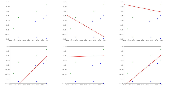
2D Model Visualization
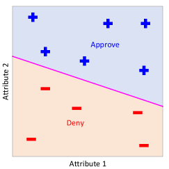
Decision boundaries: line
Decision regions: approve and deny regions
Learning Algorithm
A Simple Learning Algorithm
The performance measure: the error rate
We uses the simple learning algorithm (perceptron learning algorithm - PLA) to find {\color{red}\boldsymbol{w}} \begin{equation} \arg\min_{{\color{red}\boldsymbol{w}}}E(h_{{\color{red}\boldsymbol{w}}}(x),y\mid\mathcal{D}) \end{equation}
- Given the training set \mathcal{D}=\{(\boldsymbol{x}_{1},y_{1}),(\boldsymbol{x}_{2},y_{2}),...(\boldsymbol{x}_{N},y_{N})\}
Init \boldsymbol{{\color{red}w}}
Repeat until satisfied
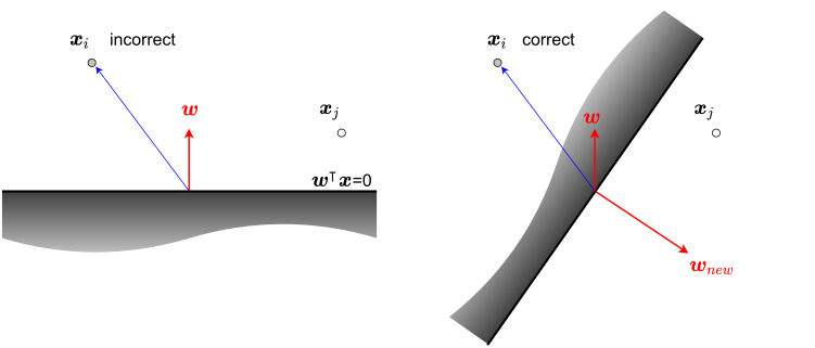
At iteration t=1,2,3,..., pick a misclassified point (\boldsymbol{x}_{i},y_{i}) \begin{equation} sign(\boldsymbol{{\color{red}w}}^{\intercal}\boldsymbol{x}_{i})\neq y_{i} \end{equation}
and update the weight vector \begin{equation} \boldsymbol{{\color{red}w}}\gets\boldsymbol{{\color{red}w}}+y_{i}\boldsymbol{x}_{i} \end{equation}
A Simple Explanation
Is It Learning Algorithm?
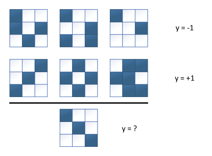
A Learning Puzzle
2.3 Feasibility Of Learning
Feasibility Of Learning
The feasibility of learning is thus split into two questions:
Can we make the performance good enough?
- run our learning algorithm on the actual data \mathcal{D} and see how good we can get.
Can we make sure that the performance inside of \mathcal{D} is close enough to the performance outside of \mathcal{D}?
- probability theory
Probability to the rescue
A Related Experiment - Bin Problem
Consider a BIN with red and green marbles \begin{align*} P[\text{picking a {\color{red}red} marble}] & =\mu\\ P[\text{picking a {\color{green}green} marble}] & =1-\mu \end{align*}
The value of \mu is unknown to us
We pick N marbles independently
The fraction of red marbles in SAMPLE = \nu
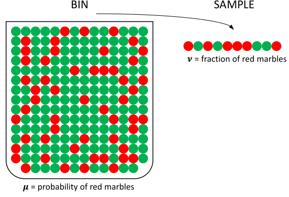
Does \nu say anything about \mu?

- No! (certain answer): Sample can be mostly red while bin is mostly red
- Yes! (uncertain answer): Sample frequency \nu is likely close to bin frequency \mu
What does \nu say about \mu?
In a big sample (large N), \nu is probably close \mu (within \epsilon)
Formally,
\begin{equation} P[|\nu-\mu|>\epsilon]\leq2e^{-2\epsilon^{2}N}\;\text{for any}\;\epsilon>0 \end{equation}This is called Hoeffding’s InequalityBound does not depend on \mu; tradeoff: N,\epsilon and the bound
We have \nu\approx\mu\Longrightarrow\mu\approx\nu
In other words, the statement “\mu=\nu” is probably approximately correct (P.A.C)
Connection to Learning
| Bin problem | Learning problem | |
| The unknown is a number \mu | The unknown is a function f:\mathcal{X}\to\mathcal{Y} | |
| a marble \circ | a point \boldsymbol{x}\in\mathcal{X} | |
| {\color{green}\circ} | hypothesis got it right h({\color{green}x})=f({\color{green}x}) | |
| {\color{red}\circ} | hypothesis got it wrong h({\color{red}x})\neq f({\color{red}x}) |
The error rate within the sample \mathcal{D}, which corresponds to \nu in the bin model, will be called the in-sample error \begin{align*} E_{in}(h) & =\text{fraction of }\mathcal{D}\text{ where }f\text{ and }h\text{ disagree}\\ & =\frac{1}{N}\sum_{n=1}^{N}\mathbb{I}(h(\boldsymbol{x}_{n})\neq f(\boldsymbol{x}_{n})) \end{align*} where \mathbb{I}(...)=1 if the statement is true, and \mathbb{I}(...)=0 if the statement is false
In the same way, we define the out-of-sample error , (domain \mathcal{X}) E_{out}(h)=P(h(\boldsymbol{x})\neq f(\boldsymbol{x})),\boldsymbol{x}\in\mathcal{X} which corresponds to \mu in the bin model.
The Hoeffding inequality becomes: \begin{equation} P[|E_{in}(h)-E_{out}(h)|>\epsilon]\leq2e^{-2\epsilon^{2}N}\;\text{for any}\;\epsilon>0 \end{equation}
2.4 Risk and Emprical Risk
Loss function
Loss function
Given a hypothesis \hat{y}=h(\boldsymbol{x})\in\mathcal{H}, a non-negative real-valued loss function \ell(\hat{y},y) which measures how different the prediction \hat{y} of a hypothesis is from the true outcome y.
Loss Functions for Binary Classification
Zero-one loss \begin{equation} \mathbb{I}(h(\boldsymbol{x})\neq y) \end{equation}
Log loss (logistic regression) \begin{equation} \log(1+e^{-h(\boldsymbol{x})y}) \end{equation}
Exponential loss (AdaBoost) \begin{equation} e^{-h(\boldsymbol{x})y} \end{equation}
Loss Functions for Regression
Squared loss \begin{equation} \left(h(\boldsymbol{x})-y\right)^{2} \end{equation}
Absolute loss \begin{equation} \left|h(\boldsymbol{x})-y\right| \end{equation}
Empirical risk
Risk
The risk E associated with hypothesis h(\boldsymbol{x}) is defined as the expectation of the loss function \begin{equation} E(h)=\mathbb{E}[\ell(h(\boldsymbol{x}),y)]=\int\ell(h(\boldsymbol{x}),y)dp(\boldsymbol{x},y) \end{equation}
Empirical Risk
The empirical risk \hat{E} is the average of the loss function on the training set \mathcal{D}=\{(\boldsymbol{x}_{1},y_{1}),(\boldsymbol{x}_{2},y_{2}),...(\boldsymbol{x}_{N},y_{N})\} \begin{equation} \hat{E}=\frac{1}{N}\sum_{i=1}^{N}\ell(h_{{\color{red}\boldsymbol{w}}}(\boldsymbol{x}_{i}),y_{i}) \end{equation}
The empirial risk is unbiased estimate of the risk
Empirical risk of hypothesis h_{{\color{red}\boldsymbol{w}}}(x) with a loss function \ell and a regularizer reg \begin{equation} \hat{E}=\frac{1}{N}\sum_{i=1}^{N}\underset{Loss}{\underbrace{\ell(h_{{\color{red}\boldsymbol{w}}}(\boldsymbol{x}_{i}),y_{i})}}+\underset{Regularizer}{\underbrace{{\color{green}\lambda}reg({\color{red}\boldsymbol{w}})}} \end{equation}
The empirical risk minimization principle
Principle The learning algorithm should choose a hypothesis h_{{\color{red}\boldsymbol{w}}} which minimizes the empirical risk \begin{equation} h_{{\color{red}\boldsymbol{w}}}=\arg\min_{h_{{\color{red}\boldsymbol{w}}}\in\mathcal{H}}\hat{E}(h_{{\color{red}\boldsymbol{w}}}\mid\mathcal{D}) \end{equation}
Regularizer
Regularizers
For each {\color{green}\lambda}\geq0, there exists B\geq0. such that the two formulations are equivalent, \begin{align} & \arg\min_{{\color{red}\boldsymbol{w}}}\sum_{i=1}^{N}\ell(h_{{\color{red}\boldsymbol{w}}}(\boldsymbol{x}_{i}),y_{i})+{\color{green}\lambda}reg({\color{red}\boldsymbol{w}})\\ & \arg\min_{{\color{red}\boldsymbol{w}}}\sum_{i=1}^{N}\ell(h_{{\color{red}\boldsymbol{w}}}(\boldsymbol{x}_{i}),y_{i})\text{ subject to }reg({\color{red}\boldsymbol{w}})\leq B \end{align}
L_{2}-regularization \begin{equation} reg({\color{red}\boldsymbol{w}})={\color{red}\boldsymbol{w}}^{\top}{\color{red}\boldsymbol{w}}=\|{\color{red}\boldsymbol{w}}\|_{2}^{2} \end{equation}
L_{1}-regularization \begin{equation} reg({\color{red}\boldsymbol{w}})=\|{\color{red}\boldsymbol{w}}\|_{1} \end{equation}