18 DEEP GENERATIVE MODELS

18.1 Generative Models

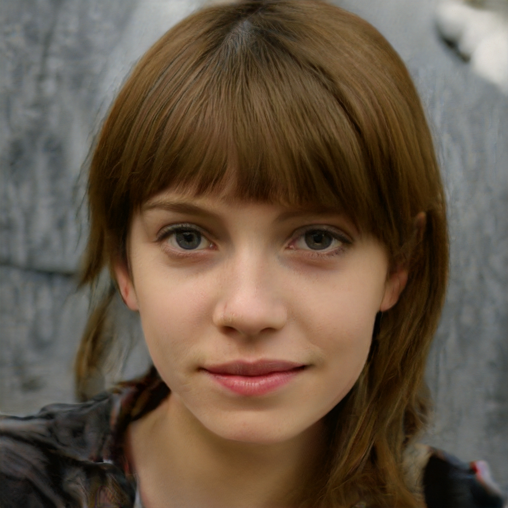
A real image?

Supervised vs unsupervised learning

Data	(x,y)	x
	x is data, y is label	x is data, no labels!
Goal	Learn function to map	Learn some hidden or underlying structure of the data
Examples	Classification, regression, object detection, semantic segmentation, etc.	Clustering, feature or dimensionality reduction, etc.

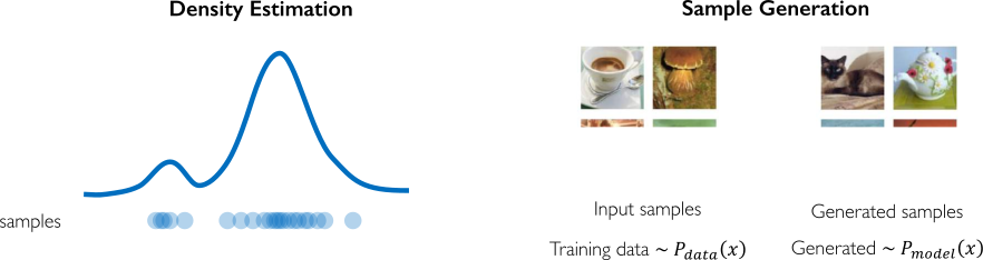
Generative modeling

Goal: Take as input training samples from some distribution and learn a model that represents that distribution
How can we learn P_{model}(x) similar to P_{data}(x)?

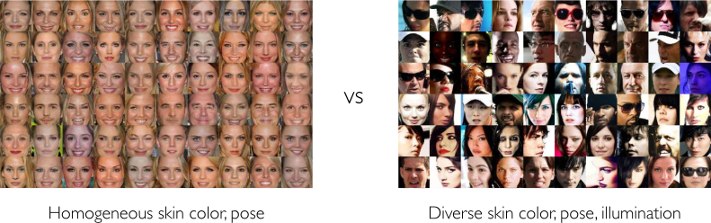
Why generative models? Debiasing

Capable of uncovering underlying latent variables in a dataset
How can we use latent distributions to create fair and representative datasets?

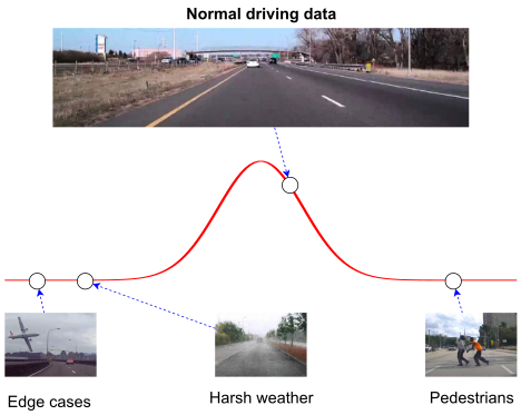
Why generative models? Outlier detection

Problem: How can we detect when we encounter something new or rare?
Strategy: Leverage generative models, detect outliers in the distribution
- Use outliers during training to improve even more!

What is a latent variable?

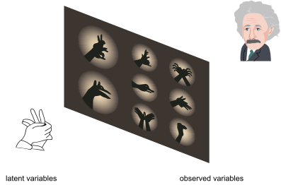
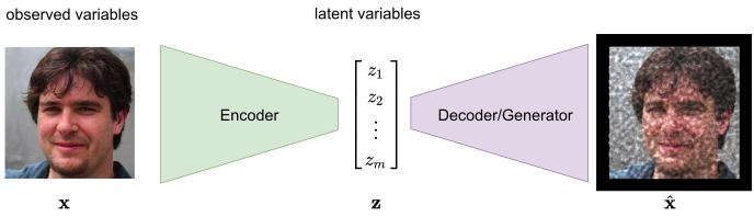
Can we learn the true explanatory factors, e.g. latent variables, from only observed data?
Latent variable model: learn a mapping from some latent variable z (or h) to a complicated distribution on x.

Discrete latent variable

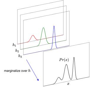
\begin{equation} Pr(x)=\sum_{i=1}^{k}Pr(x\mid h_{i})Pr(h_{i}) \end{equation}

Continuous latent variable

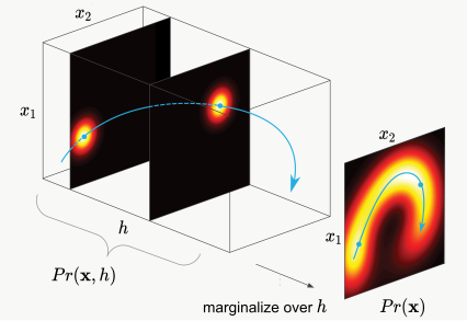
\begin{equation} Pr(x)=\int Pr(x\mid h)Pr(h)dh \end{equation}

Latent model

18.2 Autoencoders

AutoEncoder

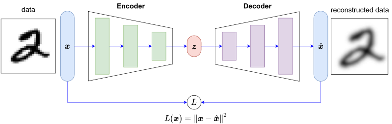
Autoencoder (automatically encoding data) is an unsupervised approach for learning a lower-dimensional feature representation from unlabeled training data

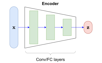
Encoder

“Encoder” learns mapping from the data, \boldsymbol{x}, to a low-dimensional latent space, \boldsymbol{z}

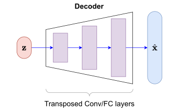
Decoder

“Decoder” learns mapping back from latent, \boldsymbol{z}, to a reconstructed observation, \hat{\boldsymbol{x}}

Loss function

How can we learn this latent space?
Train the model to use these features to reconstruct the original data
We define a loss function L (loss function doesn’t use any labels!) \begin{equation} L(\boldsymbol{x})=\left\Vert \boldsymbol{x}-\hat{\boldsymbol{x}}\right\Vert ^{2} \end{equation}

Dimensionality of latent space

Autoencoding is a form of compression!
Smaller latent space will force a larger training bottleneck

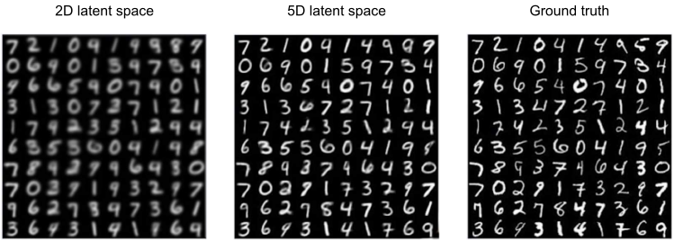
Autoencoders for representation learning

Bottleneck hidden layer forces network to learn a compressed latent representation
Reconstruction loss forces the latent representation to capture (or encode) as much “information” about the data as possible
Not probabilistic: No way to sample new data from learned model

18.3 Variational Autoencoders (VAEs)

VAEs

Variational Autoencoders

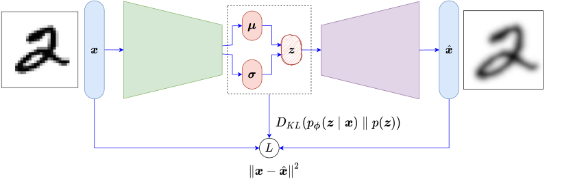
Variational autoencoders are a probabilistic twist on autoencoders!

Sample from P_{{\color{red}\boldsymbol{\phi}}}(\boldsymbol{z}\mid\boldsymbol{x}) to compute latent sample
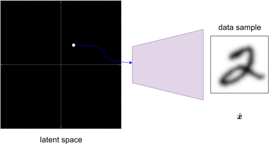
Sample from P_{{\color{red}\boldsymbol{\theta}}}(\boldsymbol{x}\mid\boldsymbol{z}) to generate data sample

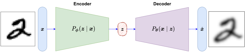
Priors on the latent distribution

Common choice of prior p(\boldsymbol{z}),\boldsymbol{z}=(z_{1},...,z_{m}): \begin{equation} \forall z_{i},\:p(z_{i})=\mathcal{N}(\mu=0,\sigma^{2}=1) \end{equation}
Encourages encodings to distribute encodings evenly around the center of the latent space
Penalize the network when it tries to “cheat” by clustering points in specific regions (ie. memorizing the data)

VAE Model

Variational autoencoders with the prior p(\boldsymbol{z})
The mean vector \boldsymbol{\mu}=(\mu_{1},...,\mu_{m})
The standard deviation vector \boldsymbol{\sigma}=(\sigma_{1},...,\sigma_{m})

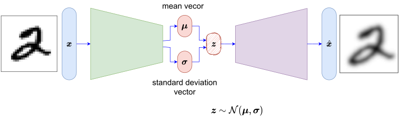
Lost function

We define a lost function L? \begin{equation} L_{{\color{red}\phi},{\color{red}\theta}}(\boldsymbol{x})=(\text{reconstruction lost})+(\text{regularization term}) \end{equation}

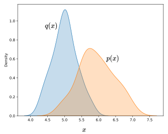
Kullback–Leibler divergence, D_{KL} (also called relative entropy), is a measure of how one probability distribution is different from a second, reference probability distribution.

For discrete probability distributions P and Q defined on the same probability space \mathcal{X} \begin{equation} D_{KL}(P\parallel Q)=\sum_{x\in\mathcal{X}}P(x)\log\left(\frac{P(x)}{Q(x)}\right) \end{equation}
For distributions P and Q of a continuous random variable \begin{equation} D_{KL}(P\parallel Q)=\int_{-\infty}^{\infty}p(x)\log\left(\frac{p(x)}{q(x)}\right)dx \end{equation}

We have \begin{align} \text{reconstruction lost} & =\left\Vert \boldsymbol{x}-\hat{\boldsymbol{x}}\right\Vert ^{2} \end{align} and \begin{align} \text{regularization term} & =D_{KL}(p_{{\color{red}\boldsymbol{\phi}}}(\boldsymbol{z}\mid\boldsymbol{x})\parallel p(\boldsymbol{z}))\\ & =D_{KL}(\mathcal{N}(\boldsymbol{\mu},\boldsymbol{\sigma})\parallel\mathcal{N}(\boldsymbol{0},\boldsymbol{1}))\\ & =-\frac{1}{2}\sum_{i=1}^{m}(\sigma_{i}+\mu_{i}^{2}-1-\log\sigma_{i}) \end{align}

VAE Optimization

Problem: The network involves a sampling step. We cannot backpropagate gradients through sampling layers!

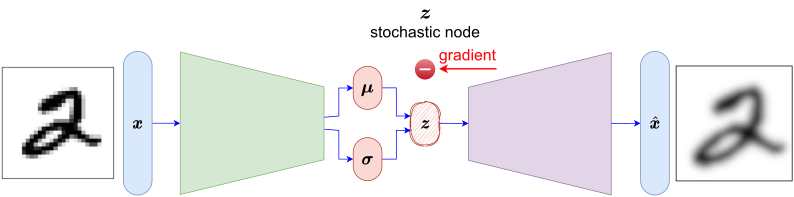
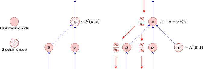
The reparameterization trick

Solution: we can move the stochastic part into a branch of the network which draws a sample \boldsymbol{\epsilon}\sim\mathcal{N}(\boldsymbol{0},\boldsymbol{1}) and then use the following formula \begin{equation} \boldsymbol{z}=\boldsymbol{\mu}+\boldsymbol{\sigma}\odot\boldsymbol{\epsilon} \end{equation}

Latent Space

Latent space

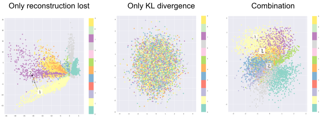
Latent space of dataset MNIST

Sampling from latent space

Latent perturbation

Slowly increase or decrease a single latent variable and keep all other variables fixed
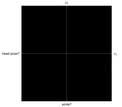
Different dimensions of \boldsymbol{z} encodes different interpretable latent features
- Ideally, we want latent variables that are uncorrelated with each other
- Enforce diagonal prior on the latent variables to encourage independence
Olivetti faces dataset
MNIST dataset

VAE summary

Compress representation of world to something we can use to learn
Reconstruction allows for unsupervised learning (no labels!)
Reparameterization trick to train end-to-end
Interpret hidden latent variables using perturbation
Generating new examples

18.4 Generative Adversarial Networks (GANs)

What if we just want to sample?

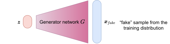
Idea: don’t explicitly model density, and instead just sample to generate new instances.
Problem: want to sample from complex distribution – can’t do this directly!
Solution: sample from something simple (noise), learn a transformation to the training distribution.

Generative Adversarial Networks (GANs)

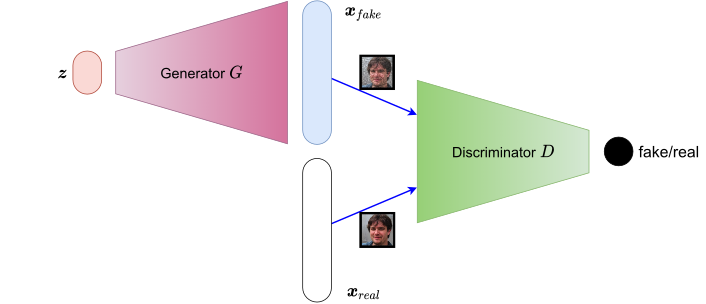
Generative Adversarial Networks (GANs) are a way to make a generative model by having two neural networks compete with each other.

The generator D turns noise into an imitation of the data to try to trick the discriminator.
The discriminator G tries to identify real data from fakes created by the generator.

GAN objective

Expected conditional log likelihood for real and generated data \begin{equation} V(G,D)=\underset{\text{real data}}{\underbrace{\mathbb{E}_{\boldsymbol{x}\sim p(\text{data})}\log D_{{\color{red}\boldsymbol{\theta}_{d}}}(\boldsymbol{x})}}+\underset{\text{generated data}}{\underbrace{\mathbb{E}_{\boldsymbol{z}\sim p(\boldsymbol{z})}\log(1-D_{{\color{red}\boldsymbol{\theta}_{d}}}(G_{{\color{red}\boldsymbol{\theta}_{g}}}(\boldsymbol{z})))}} \end{equation}
The discriminator wants to correctly distinguish real and fake samples \begin{equation} D^{\ast}=\arg\max_{D}V(G,D) \end{equation}
The generator wants to fool the discriminator \begin{equation} G^{\ast}=\arg\min_{G}V(G,D) \end{equation}

Training GANs

Discriminator tries to identify real data from fakes created by the generator.
Generator tries to create imitations of data to trick the discriminator.

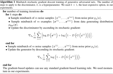
Train GAN jointly via minimax game \begin{equation} \arg\min_{{\color{red}\boldsymbol{\theta}_{g}}}\max_{{\color{red}\boldsymbol{\theta}_{d}}}\left[\mathbb{E}_{\boldsymbol{x}\sim p(\text{data})}\log D_{{\color{red}\boldsymbol{\theta}_{d}}}(\boldsymbol{x})+\mathbb{E}_{\boldsymbol{z}\sim p(\boldsymbol{z})}\log(1-D_{{\color{red}\boldsymbol{\theta}_{d}}}(G_{{\color{red}\boldsymbol{\theta}_{g}}}(\boldsymbol{z})))\right] \end{equation}

Discriminator wants to maximize objective s.t. D(\boldsymbol{x}) close to 1, D(G(\boldsymbol{z})) close to 0.
Generator wants to minimize objective s.t. D(G(\boldsymbol{z})) close to 1

Algorithm

Training in practice

The minimax objective leads to vanishing gradients as the discriminator saturates.
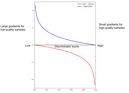
In practice, Goodfellow et al (2014) advocate the heuristic training objective:
Discriminator

\begin{equation} \arg\max_{{\color{red}\boldsymbol{\theta}_{d}}}\left[\mathbb{E}_{\boldsymbol{x}\sim p(\text{data})}\log D_{{\color{red}\boldsymbol{\theta}_{d}}}(\boldsymbol{x})+\mathbb{E}_{\boldsymbol{z}\sim p(\boldsymbol{z})}\log(1-D_{{\color{red}\boldsymbol{\theta}_{d}}}(G_{{\color{red}\boldsymbol{\theta}_{g}}}(\boldsymbol{z})))\right] \end{equation}

Generator

\begin{equation} \arg\max_{{\color{red}\boldsymbol{\theta}_{g}}}\left[\mathbb{E}_{\boldsymbol{z}\sim p(\boldsymbol{z})}\log(D_{{\color{red}\boldsymbol{\theta}_{d}}}(G_{{\color{red}\boldsymbol{\theta}_{g}}}(\boldsymbol{z})))\right] \end{equation}

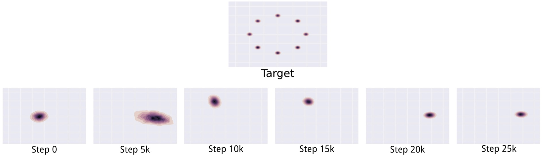
Generating new data with GANs

After training, use generator network to create new data that’s never been seen before.

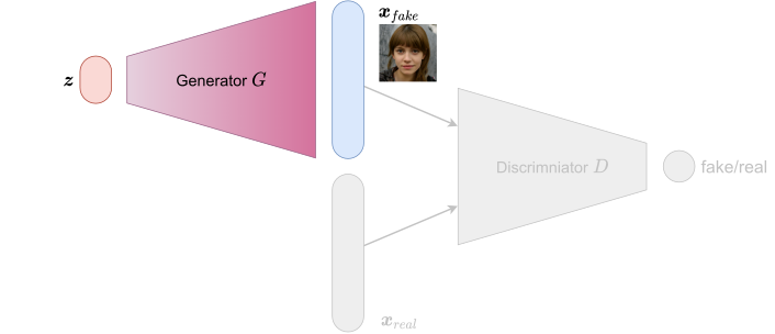
18.5 GAN Evaluation

18.6 GAN Recent Advances

Progressive GANs (NVIDIA)

Key idea: train lower-resolution models, gradually add layers corresponding to higher-resolution outputs (Karras et al., ICLR 2018.)

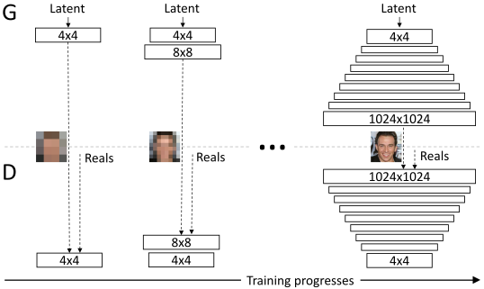
Progressive GANs: results

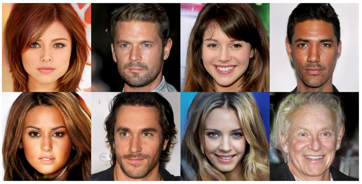
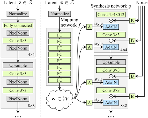
StyleGAN

Built on top of Progressive GAN
Start with learned constant (instead of noise vector)
Use a mapping network to produce a style code \boldsymbol{w} using learned affine transformations A
Use adaptive instance normalization (AdaIN): scale and bias each feature map using learned style values
Add noise after each convolution and before nonlinearity (enables stochastic detail)

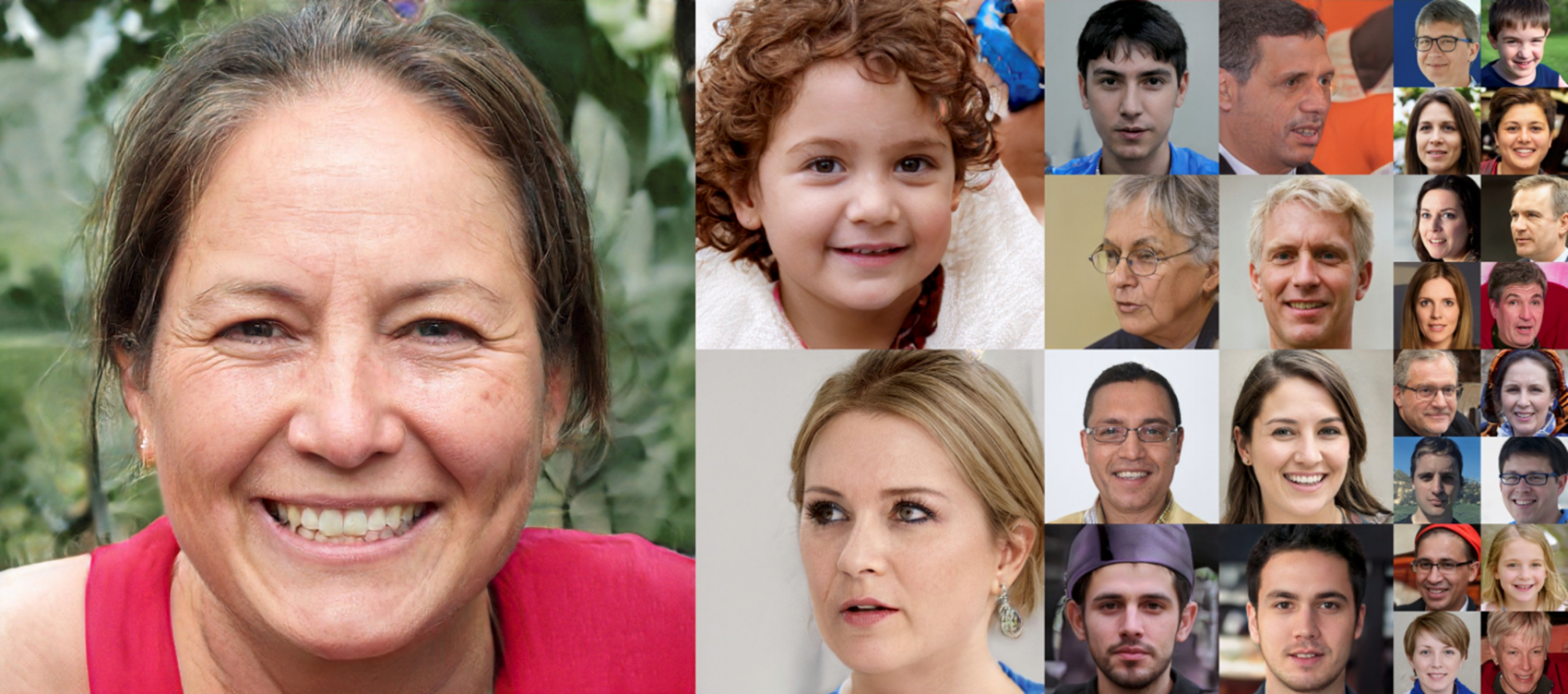
StyleGAN: results

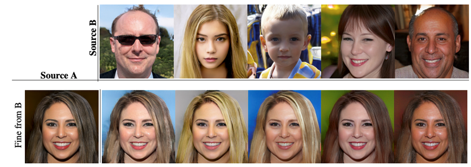
Mixing styles

Two sets of images were generated from their respective latent codes (sources A and B); the rest of the images were generated by copying a specified subset of styles from source B and taking the rest from source A.

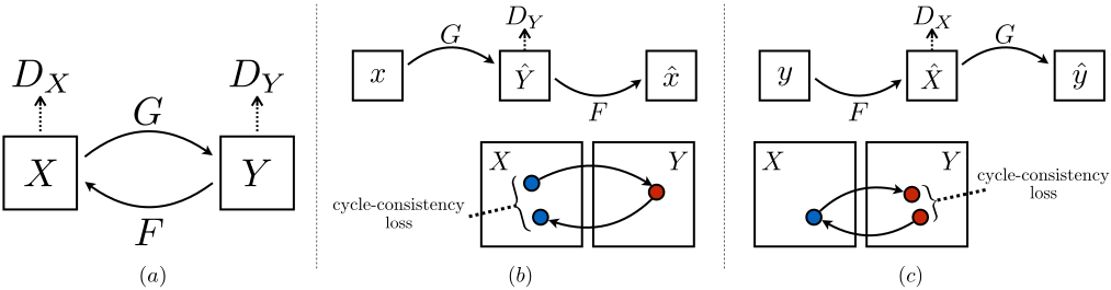
CycleGAN

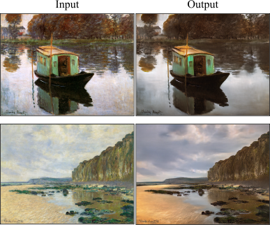
CycleGAN learns transformations across domains with unpaired data.