12 SUPPORT VECTOR MACHINE
12.1 Linear Support Vector Machines
The Separable Case
Problem Statement
Training set: (\boldsymbol{x}_{i},y_{i})_{i=1...N}\in\mathbb{R}^{D}\times\left\{ -1,1\right\}
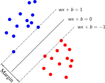
We would like to find an hyperplane {\color{red}\boldsymbol{w}}^{\intercal}\boldsymbol{x}+{\color{red}b}=0,\quad({\color{red}\boldsymbol{w}}\in\mathbb{R}^{D},{\color{red}b}\in\mathbb{R}) which separates the two classes.
Margin
Let d_{+} be the shortest distance from the hyperplane to the closest positive example.
Let d_{-} be the shortest distance from the hyperplane to the closest negative example.
Define the margin of the hyperplane to be \min(d_{+},d_{-}).
Better Linear Separation
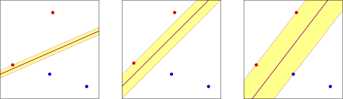
Two questions:
Why is bigger margin better?
Which {\color{red}\boldsymbol{w}},{\color{red}b} maximizes the margin
Why is it Good to Maximize the Margin?
If training and test data come from the same distribution and all test data are within some \Delta distance from the training points. If all points lie at a distance of at least \Delta from the separator, and all points are in a bounded sphere, then a small perturbation of the definition of the separator will not hurt.

One can use less bits to encode the separating hyperplane (Minimum Description Length principle)

Finding \boldsymbol{w} with large margin
Let \boldsymbol{x}_{n} be the nearest data point to the plane {\color{red}\boldsymbol{w}}^{\intercal}\boldsymbol{x}+{\color{red}b}=0. How far is it?
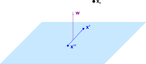
The distance between \boldsymbol{x}_{n} and the plane {\color{red}\boldsymbol{w}}^{\intercal}\boldsymbol{x}+{\color{red}b}=0 where \left|{\color{red}\boldsymbol{w}}^{\intercal}\boldsymbol{x}_{n}+{\color{red}b}\right|=1 (normalize {\color{red}\boldsymbol{w}} and b) \begin{equation} distance=\frac{1}{\left|{\color{red}\boldsymbol{w}}\right|} \end{equation}
A Constrained Optimization Problem
Representation of hypothesis set \begin{equation} \mathcal{H}:y=f(\boldsymbol{x})=\text{sign}({\color{red}\boldsymbol{w}}\cdot\boldsymbol{x}+{\color{red}b}) \end{equation}
Evaluation
\begin{align} & \arg\min_{{\color{red}\boldsymbol{w}},{\color{red}b}} & \frac{1}{2}\|{\color{red}\boldsymbol{w}}\|^{2}\\ & \text{subject to} & y_{i}({\color{red}\boldsymbol{w}}\cdot\boldsymbol{x}_{i}+{\color{red}b})\geq1,\quad i=1,2,\dots,N \end{align}
The Dual Formulation
Representation of hypothesis set \begin{equation} \mathcal{H}:y=f(\boldsymbol{x})=\text{sign}\left(\sum\limits_{i=1}^{N}{\color{red}\alpha_{i}}y_{i}(\boldsymbol{x}\cdot\boldsymbol{x}_{i})+{\color{red}b}\right) \end{equation}
Evaluation \begin{align} & \arg\min_{{\color{red}\boldsymbol{\alpha}}} & \frac{1}{2}\sum\limits_{i=1}^{N}\sum\limits_{j=1}^{N}{\color{red}\alpha_{i}\alpha_{j}}y_{i}y_{j}(\boldsymbol{x}_{i}\cdot\boldsymbol{x}_{j})-\sum\limits_{i=1}^{N}{\color{red}\alpha_{i}}\\ & \text{subject to} & \sum\limits_{i=1}^{N}{\color{red}\alpha_{i}}y_{i}=0\\ & & {\color{red}\alpha_{i}}\geq0,\quad i=1,2,\dots,N \end{align}
This can be solved using classical quadratic programming optimization
The Non-Separable Case
Bug
- This minimization problem does not have any solution if the two classes are not separable.
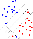
Fixing The Bug: “Soft” Margin
Relax the constraints: use a soft margin instead of a hard margin.
We would like to minimize:
\begin{align} & \arg\min_{{\color{red}\boldsymbol{w}},{\color{red}b},{\color{red}\boldsymbol{\xi}}} & \frac{1}{2}\|{\color{red}\boldsymbol{w}}\|^{2}+{\color{green}C}\sum\limits_{i=1}^{N}{\color{red}\xi_{i}}\\ & \text{subject to} & y_{i}({\color{red}\boldsymbol{w}}\cdot\boldsymbol{x}_{i}+{\color{red}b})\geq1-{\color{red}\xi_{i}}\\ & & {\color{red}\xi_{i}}\geq0,\quad i=1,2,\dots,N \end{align}
The Dual Formulation
Representation of hypothesis set \begin{equation} \mathcal{H}:y=f(\boldsymbol{x})=\text{sign}\left(\sum\limits_{i=1}^{N}{\color{red}\alpha_{i}}y_{i}(\boldsymbol{x}\cdot\boldsymbol{x}_{i})+{\color{red}b}\right) \end{equation}
Evaluation \begin{align} & \arg\min_{{\color{red}\boldsymbol{\alpha}}} & \frac{1}{2}\sum\limits_{i=1}^{N}\sum\limits_{j=1}^{N}{\color{red}\alpha_{i}\alpha_{j}}y_{i}y_{j}(\boldsymbol{x}_{i}\cdot\boldsymbol{x}_{j})-\sum\limits_{i=1}^{N}{\color{red}\alpha_{i}}\\ & \text{subject to} & \sum\limits_{i=1}^{N}{\color{red}\alpha_{i}}y_{i}=0\\ & & 0\leq{\color{red}\alpha_{i}}\leq{\color{green}C},\quad i=1,2,\dots,N \end{align}
Support Vector Terminology
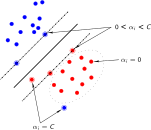
- Training examples \boldsymbol{x}_{i} with \alpha_{i}>0 are support vectors. \begin{align} {\color{red}\alpha_{i}}=0\Rightarrow y_{i}({\color{red}\boldsymbol{w}}\cdot\boldsymbol{x}_{i}+{\color{red}b})>1\nonumber \\ {\color{red}\alpha_{i}}={\color{green}C}\Rightarrow y_{i}({\color{red}\boldsymbol{w}}\cdot\boldsymbol{x}_{i}+{\color{red}b})<1\\ 0<{\color{red}\alpha_{i}}<{\color{green}C}\Rightarrow y_{i}({\color{red}\boldsymbol{w}}\cdot\boldsymbol{x}_{i}+{\color{red}b})=1\nonumber \end{align}
12.2 Kernels Support Vector Machines
Non-Linear SVMs
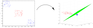
Project the data into a higher dimensional space (feature space): it should be easier to separate the two classes.
Given a function \phi:\mathbb{R}^{D}\to\mathcal{F}, work with \phi(\boldsymbol{x}_{i}) instead of working with \boldsymbol{x}_{i}.
The Kernel Function
A kernel is a function k(\boldsymbol{x},\boldsymbol{z}) which represents a dot product in a “hidden” feature space of \phi. \begin{equation} k(\boldsymbol{x},\boldsymbol{z})=\phi(\boldsymbol{x})\cdot\phi(\boldsymbol{z}) \end{equation}
Note that: we have only dot products \phi(\boldsymbol{x}_{i})\cdot\phi(\boldsymbol{x}_{j}) to compute; however, this could be very expensive in a high dimensional space.
Kernel trick:
instead of \phi(\boldsymbol{x})=\phi\left(\begin{array}{c} x_{1}\\ x_{2} \end{array}\right)=\left(\begin{array}{c} x_{1}^{2}\\ \sqrt{2}x_{1}x_{2}\\ x_{2}^{2} \end{array}\right), use k(\boldsymbol{x},\boldsymbol{z})=(\boldsymbol{x}\cdot\boldsymbol{z})^{2}
Common Kernels
Polynomial: \begin{equation} k(\boldsymbol{x},\boldsymbol{z})=(u\boldsymbol{x}\cdot\boldsymbol{z}+v)^{p}\;(u\in\mathbb{R},v\in\mathbb{R},p\in\mathbb{N}) \end{equation}
Gaussian: \begin{equation} k(\boldsymbol{x},\boldsymbol{z})=\exp\left(-\frac{\left\Vert \boldsymbol{x}-\boldsymbol{z}\right\Vert ^{2}}{{\color{green}\sigma}^{2}}\right)\;,{\color{green}\sigma}\in\mathbb{R}^{+} \end{equation}
Techniques for Construction of Kernels
In all the following, k_{1},k_{2},...,k_{j} are assumed to be valid kernel functions
Scalar multiplication: The validity of a kernel is conserved after multiplication by a positive scalar, i.e., for any \alpha>0, the function \begin{equation} k(\boldsymbol{x},\boldsymbol{z})=\alpha k_{1}(\boldsymbol{x},\boldsymbol{z}) \end{equation}
Adding a positive constant: For any positive constant \alpha>0, the function \begin{equation} k(\boldsymbol{x},\boldsymbol{z})=\alpha+k_{1}(\boldsymbol{x},\boldsymbol{z}) \end{equation}
Linear combination: A linear combination of kernel functions involving only positive weights, i.e., \begin{equation} k(\boldsymbol{x},\boldsymbol{z})=\sum_{j=1}^{m}\alpha_{j}k_{j}(\boldsymbol{x},\boldsymbol{z}),\qquad\text{with }\alpha_{j}>0 \end{equation} is a valid kernel function.
Product: The product of two kernel functions, i.e., \begin{equation} k(\boldsymbol{x},\boldsymbol{z})=k_{1}(\boldsymbol{x},\boldsymbol{z})k_{2}(\boldsymbol{x},\boldsymbol{z}) \end{equation} is a valid kernel function.
Polynomial functions of a kernel output: Given a polynomial f:\mathbb{R}\to\mathbb{R} with positive coefficients, the function \begin{equation} k(\boldsymbol{x},\boldsymbol{z})=f(k_{1}(\boldsymbol{x},\boldsymbol{z})) \end{equation} is a valid kernel function.
Exponential function of a kernel output: The function \begin{equation} k(\boldsymbol{x},\boldsymbol{z})=\exp(k_{1}(\boldsymbol{x},\boldsymbol{z})) \end{equation} is a valid kernel function.
Product of matrix and vectors: \begin{equation} k(\boldsymbol{x},\boldsymbol{z})=\boldsymbol{x}^{\intercal}A\boldsymbol{z} \end{equation} where A is a symmetric positive semidefinite matrix.
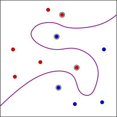
Decision Boundary and Support Vectors
SVMs in Practice
In order to tune the capacity, the kernel is the most important parameter to choose.
Polynomial kernel: increasing the degree will increase the capacity.
Gaussian kernel: increasing {\color{green}\sigma} will decrease the capacity.
Tune {\color{green}C}, the trade-off between the margin and the errors.
For non-noisy data sets, {\color{green}C} usually has not much influence.
Carefully choose {\color{green}C} for noisy data sets: small values usually give better results.
12.3 Multi-class SVM
Multiclass SVM formulations
There are a few ways of formulating the SVM over multiple classes:
One-vs-all
One-vs-one
Hierarchical
Multiclass
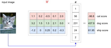
Score function
The score function f that maps the raw features to class scores. \begin{equation} \boldsymbol{z}=f(\boldsymbol{x};{\color{red}W})={\color{red}W}\boldsymbol{x} \end{equation}
Multiclass SVM loss
- Given the input vector \boldsymbol{x}_{i} and the label y_{i} that specifies the index of the correct class. The multiclass SVM loss (hinge loss) for the vector \boldsymbol{x}_{i} is then formalized as follows \begin{equation} L_{i}=\sum_{j\neq y_{i}}\max(0,z_{j}-z_{y_{i}}+{\color{green}\Delta}) \end{equation} where \boldsymbol{z}=f(\boldsymbol{x}_{i};{\color{red}W})={\color{red}W}\boldsymbol{x}_{i}
Example
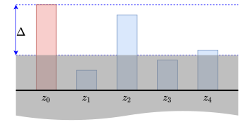
Suppose that we have five classes \{0,1,2,3,4\} that receive the scores \boldsymbol{z}=[17,4,15,6,8] and the true class y_{i}=0
Also assume that {\color{green}\Delta}=10
\begin{align*} L_{i} & =\max(0,4-17+10)+\max(0,15-17+10)\\ & +\max(0,6-17+10)+\max(0,8-17+10)=9 \end{align*}
Regularization loss
The most common regularization penalty is the L_{2} norm that discourages large weights through an elementwise quadratic penalty over all parameters: \begin{equation} R(W)=\sum_{k}\sum_{l}{\color{red}W}_{k,l}^{2} \end{equation}
The data loss (which is the average loss L_{i} over all examples) and the regularization loss. That is, the full multiclass SVM loss becomes: \begin{equation} \mathcal{L}=\mathcal{L}_{\text{data}}+\mathcal{L}_{\text{reg}}=\underbrace{\frac{1}{N}\sum_{i}L_{i}}_{\text{data loss}}+\underbrace{{\color{green}\lambda}R({\color{red}W})}_{\text{regularization loss}} \end{equation}
Learning goal: Find {\color{red}W} that minimize \begin{equation} \arg\min_{{\color{red}W}}\mathcal{L} \end{equation}
Practical considerations
Setting Delta: It can safely be set to {\color{green}\Delta}=1.0 in all cases
Relation to Binary Support Vector Machine: The loss for the i-th example (\boldsymbol{x}_{i},y_{i}) can be written as \begin{equation} L_{i}={\color{green}C}\max(0,1-y_{i}{\color{red}\boldsymbol{w}}^{\intercal}\boldsymbol{x}_{i})+R({\color{red}\boldsymbol{w}}) \end{equation} where {\color{green}C} is a hyperparameter, and y_{i}\in\{-1,1\}
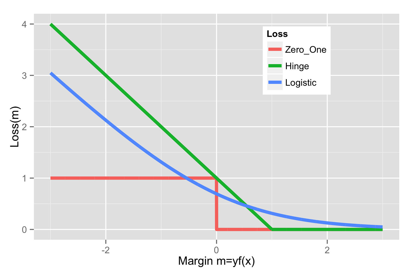
Binary classification losses
Perceptron (zero-one)
SVM (hinge)
Logistic
SGD for hinge loss
Consider linear hypothesis space: \begin{equation} h_{{\color{red}\boldsymbol{w}}}(\boldsymbol{x})={\color{red}\boldsymbol{w}}^{\intercal}\boldsymbol{x} \end{equation}
Hinge loss of (\boldsymbol{x},y) \begin{equation} \mathcal{L}(x)=\max(0,1-y{\color{red}\boldsymbol{w}}^{\intercal}\boldsymbol{x}) \end{equation}
Gradient of hinge loss (\boldsymbol{x},y): \begin{equation} \nabla_{{\color{red}\boldsymbol{w}}}\mathcal{L}(\boldsymbol{x})=\begin{cases} -y\boldsymbol{x} & \text{if }yh_{{\color{red}\boldsymbol{w}}}(\boldsymbol{x})<1\\ 0 & \text{if }yh_{{\color{red}\boldsymbol{w}}}(\boldsymbol{x})>1\\ \text{undefined} & \text{if }yh_{{\color{red}\boldsymbol{w}}}(\boldsymbol{x})=1 \end{cases} \end{equation}
A point with margin m=yh_{{\color{red}\boldsymbol{w}}}(\boldsymbol{x})=1 is correctly classified \to we can skip SGD update for these points.