15 CONVOLUTIONAL NEURAL NETWORKS
15.1 Architecture
Convolutional neural network
Convolutional neural networks (CNNs) use three basic ideas:
local receptive fields
shared weights
pooling
What are learnt in CNNs?
CNNs has two interesting properties
The patterns they learn are translation invariant
They can learn spatial hierarchies of patterns
A basic architecture of CNN
A common pattern
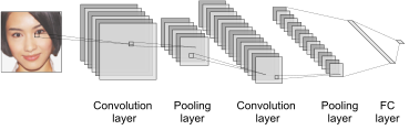
Convolution + ReLU \to Pool \to Fully connected \to Softmax loss
15.2 Convolutional layer
Convolutional layer
The fundamental difference between a densely connected layer and a convolution layer is this:
Dense layers learn global patterns in their input feature space
Convolutional layers learn local patterns in their input feature space
Convolutional types
There are three common kinds of convolution
1D convolution
2D convolution
3D convolution
Single Input, Single Output
Image processing
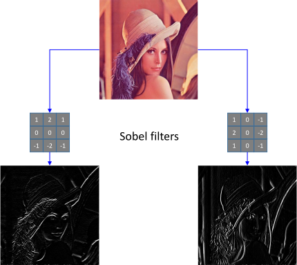
In image processing, an input image is convolved with a kernel to create an output image
Input image (input feature map) In
Output image (output feature map) Out
Filter (kernel) requires three parameters
The spatial extent (kernel size) F
The stride S (distance between two consecutive positions of the kernel)
The amount of zero padding P (number of zeros concatenated at the beginning and at the end of an axis)
Convolution vs. Cross-correlation
- Convolution operation (used in digital processing)
\begin{equation} Out(x,y)=(K*In)(x,y)=\sum_{m}\sum_{n}In(x-m,y-n)K(m,n) \end{equation}
- Cross-correlation operation (used in CNN)
\begin{equation} Out(x,y)=(K*In)(x,y)=\sum_{m}\sum_{n}In(x+m,y+n)K(m,n) \end{equation}
The following figure illustrates 2D cross-correlation operation.
Input size is 3\times3
Output size is 2\times2
Kernel has F=2,S=1,P=0
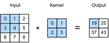
The shaded portions are the first output element as well as the input and kernel tensor elements used for the output computation 0\times0+1\times1+3\times2+4\times3=19
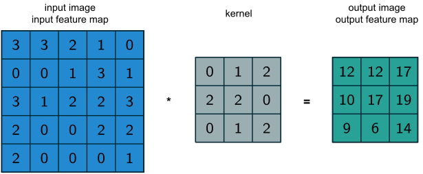
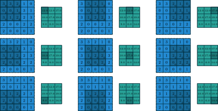
Example 1
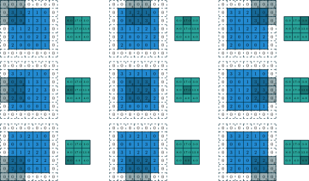
Input image size is 5\times5
Output image size is 3\times3
Kernel has F=3,S=1,P=0
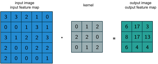
Example 2
Input image size is 5\times5
Output image size is 3\times3
Kernel has F=3,S=2,P=1
Multiple Input, Multiple Output
Multiple Input Channels
- Convolution computation with 2 input channels.
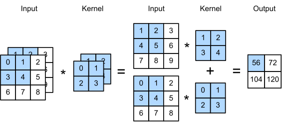
- The shaded portions are the first output element as well as the input and kernel tensor elements used for the output computation (1\times1+2\times2+4\times3+5\times4)+(0\times0+1\times1+3\times2+4\times3)=56
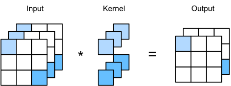
Multiple Input, Output Channels
- Convolution computation for 3 input channels and 2 output channels.
Tensor Operation
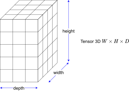
3D tensor
- Convolutions operate over 3D tensors, called feature maps, with two spatial axes (width W and height H) as well as a depth axis D (also called the channels axis)
Convolution operator
Accepts a volume of size W_{in}\times H_{in}\times D_{in} and a group of filters with four hyperparameters:
Number of filters K
Their spatial extent F
The stride S
The amount of zero padding P
- Produces a volume of size W_{out}\times H_{out}\times D_{out} where: \begin{align} W_{out} & =\frac{W_{in}-F+2P}{S}+1\nonumber \\ H_{out} & =\frac{H_{in}-F+2P}{S}+1\nonumber \\ D_{out} & =K \end{align}
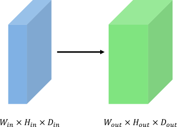
In summary,
With parameter sharing, it introduces F\times F\times D_{in} weights per filter, for a total of F\times F\times D_{in}\times K weights and K biases.
The filters depth is always equal to the input volume depth.
The output volume depth is equal to the number of filters
In the output volume, the d-th depth slice (of size W_{out}\times H_{out} is the result of performing a valid convolution of the d-th filter over the input volume with a stride of S, and then offset by d-th bias.
Normally, in the same conv layer, all filters have the same dimensions so that special optimized routines can be invoked.
Explanation
We can imagine a filter as a neuron.
In a convolution layer we have filters.
Each filter is a weight matrix which is convoluted over the input volume.
Each time the filter is applied it outputs a single value.
The result of convolving the filter over all the input volume (input feature maps) is another volume called activation map (output feature map).
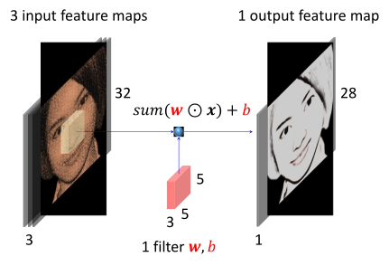
A filter’s depth is always equal to the input volume depth.
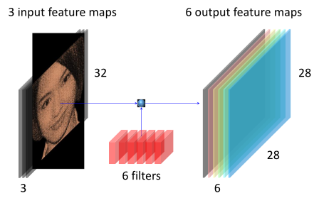
Instead of having only one filter, we have a stack of filter which produce a stack of activation maps (one for each filter)
The input volume 32\times32\times3 is convolved with the filter 5\times5\times3 (S=1 and P=0) and the result is the activation map 28\times28\times1
The input volume 32\times32\times3 is convolved with the stack of 6 filter 5\times5\times3 and the result is the stack of 6 activation map 28\times28\times1 (28\times28\times6)
15.3 Pooling layer
Pooling layer
The reason to use pooling layer (downsampling) is to reduce the number of feature-map coefficients to process
Pooling layers also provide invariance to small translations of the input
The most common kind of pooling is max pooling
Another kind of pooling is average pooling; however, it’s more informative to look at the maximal presence of different features than at their average presence
Pooling operator
Accepts a volume of size W_{in}\times H_{in}\times D_{in} and one filter with two hyperparameters:
Their spatial extent F
The stride S
Produces a volume of size W_{out}\times H_{out}\times D_{out} where: \begin{align} W_{out} & =\frac{W_{in}-F}{S}+1\nonumber \\ H_{out} & =\frac{H_{in}-F}{S}+1\nonumber \\ D_{out} & =D_{in} \end{align}
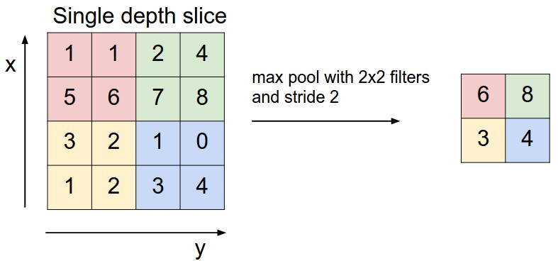
The most common form is the filter of size 2\times2 applied with a stride of 2.
Example
The input volume of size [224\times224\times64] is pooled with filter size 2, stride 2 into output volume of size [112\times112\times64]
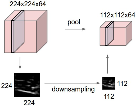
Max pooling with filter size 2, stride 2
15.4 Fully connected layer
Fully connected layer
Fully connected layers (FC layers), also called affine layers, produce the high-level reasoning in the DNN.
Neurons in a fully connected layer have full connections to all activations in the previous layer, as in regular Neural Networks.
Their activations can hence be computed with a matrix multiplication followed by a bias offset.
VGGNet
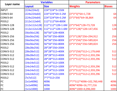
Total variables (memory): 24M \times 4 bytes \simeq 93MB/image (only forward! \sim\times2 for backward)
Total parameters: 138M parameters
The most of the network parameters are in the FC layer and most of the variables (memory) required by the network is used in the first 2 Conv Layers.
15.5 Visualizing and Understanding
First Layer
Visualize first-layer filters/kernels (raw weights) directly
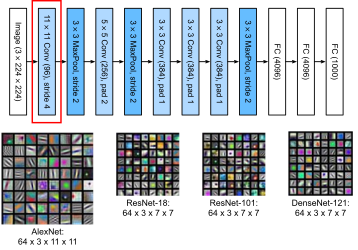
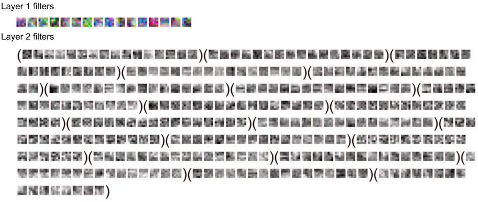
We can visualize filters at higher layers, but not that interesting (these pictures are taken from ConvNetJS CIFAR-10 demo)
Last Layer
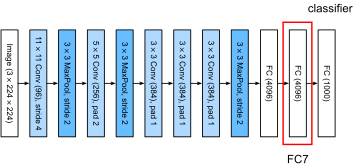
FC7: 4096-dimensional feature vector for an image (layer immediately before the classifier)
Run the network on many images, collect the feature vectors
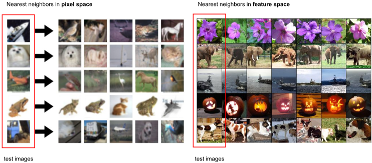
Last Layer: Nearest Neighbors
Last Layer: Dimensionality Reduction
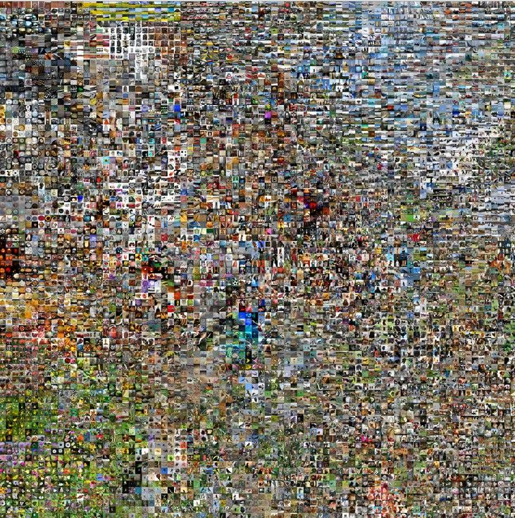
Visualize the “space” of FC7 feature vectors by reducing dimensionality of vectors from 4096 to 2 dimensions
Simple algorithm: Principal Component Analysis (PCA)
More complex: t-SNE
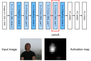
Visualizing Activations
- A view of the 13\times13 activation of the 151^{st} channel on the conv5 layer
Mapping activations back to pixels
(Guided) backpropagation method
Which pixels matter: Saliency
Compute gradient of (unnormalized) class score with respect to image pixels,
Take absolute value and max over RGB channels
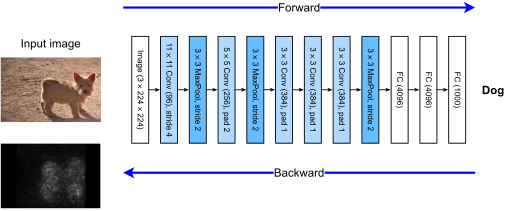
Superimposing the class activation heatmap on the original picture

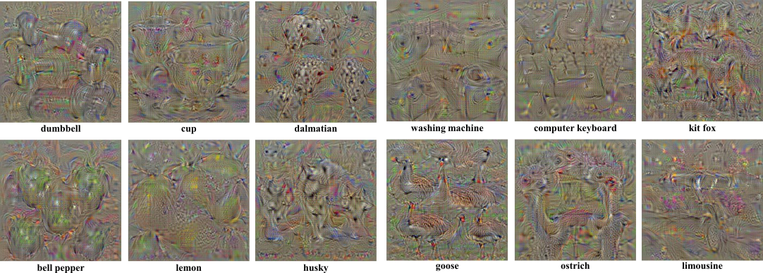
Generate Images: Gradient Ascent
| (Guided) backpropagation | Gradient ascent |
| Find the part of an image that a neuron responds to | Generate a synthetic image that maximally activates a neuron |
\begin{equation} I_{syn}=\arg\max_{I}S_{c}(I)-\lambda\left\Vert I\right\Vert _{2}^{2} \end{equation} where S_{c} score for class c (before Softmax)
Generate Images: Gradient Ascent
15.6 Network Design
Networks Using Blocks
Blocks
The design of neural network architectures had grown progressively more abstract, moving from thinking in terms of individual neurons to whole layers, and now to blocks, repeating patterns of layers.
The basic building block of classic CNNs is a sequence of the following:
a convolutional layer with padding to maintain the resolution
a nonlinearity such as a ReLU
a pooling layer such as a max pooling layer
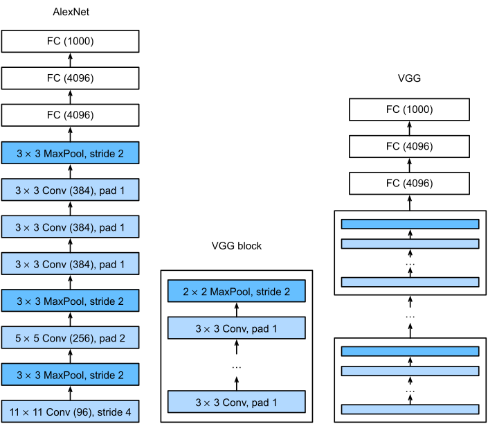
VGG Network
- From AlexNet to VGG that is designed from building blocks.
Networks with Parallel Concatenations
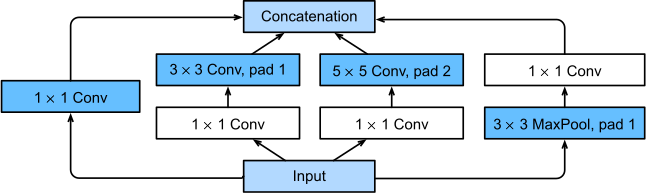
Inception Blocks
- Inception block employs a combination of variously-sized kernels
GoogleNet
- GoogLeNet uses a stack of a total of 9 inception blocks and global average pooling to generate its estimates.
Residual Networks
Learning Model
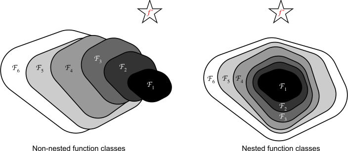
Consider \mathcal{F}, the class of functions (hypothesis set) that a specific network architecture can reach.
Given a data set \mathcal{D}, algorithm A finds the best estimated \hat{f} of the “truth” function f^{\ast}
\begin{align} \hat{f}=\arg\min_{f}L(f\mid\mathcal{D})\text{ subject to }f & \in\mathcal{F}. \end{align}
For non-nested function classes, a larger (indicated by area) function class does not guarantee to get closer to the “truth” function f^{\ast}. This does not happen in nested function classes.
Residual Blocks
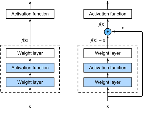
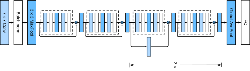
A regular block (left) and a residual block (right).
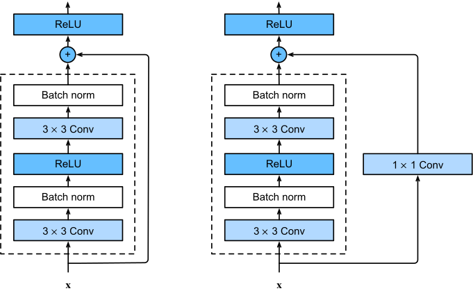
ResNet block with and without 1\times1 convolution.
ResNet Model
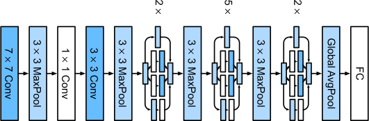
The ResNet-18 architecture
15.7 Miscellaneous convolutions
Transposed convolution
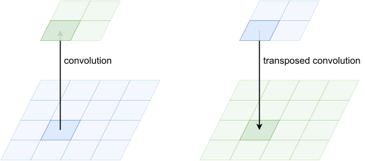
Transposed convolution
Convolution can be interpreted as a matrix multiplication \text{kernel}\;w\to\text{matrix}\;C
The need for transposed convolutions (often called deconvolution) generally arises from the desire to use a transformation going in the opposite direction of a normal convolution \text{convolution}\;C\longleftrightarrow\text{transposed convolution}\;C^{\intercal}
No zero padding, unit strides, transposed
convolution transposed convolution kernel size k k'=k stride s=1 s'=1 padding p=0 p'=k-1 output size o'=i'+(k-1) 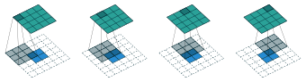
Zero padding, unit strides, transposed
convolution transposed convolution kernel size k k'=k stride s=1 s'=1 padding p p'=k-p-1 output size o'=i'+(k-1)-2p 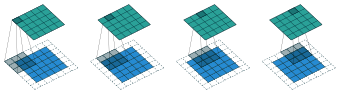
No zero padding, non-unit strides, transposed:
adding s-1 zeros between each input unit
** convolution** ** transposed convolution** kernel size k k'=k stride s s'=1 padding p=0 p'=k-1 output size o'=s(i'-1)+k 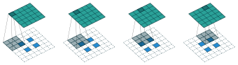
Dilated convolutions
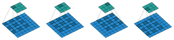
Dilated convolutions
Dilated convolutions “inflate” the kernel by inserting spaces between the kernel elements. The dilation “rate” is controlled by an additional hyperparameter d.
- For any i, k, s and p, and for a dilation rate d, \begin{equation} o=\left\lfloor \frac{i+2p-k-(k-1)(d-1)}{s}\right\rfloor +1. \end{equation}
15.8 Applications
Datasets
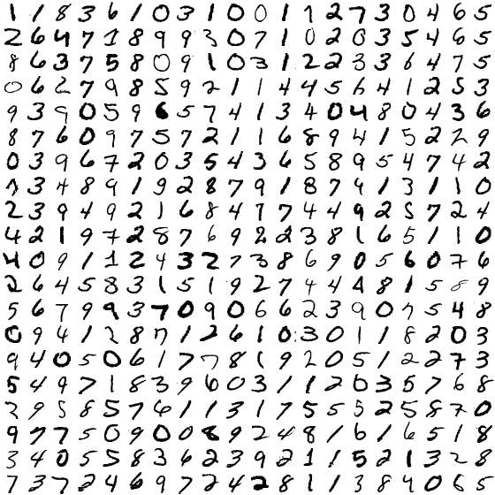
MNIST
The MNIST database is a large database of handwritten digits that is commonly used for training various image processing systems
The MNIST database contains 60,000 training images and 10,000 testing images
CIFAR
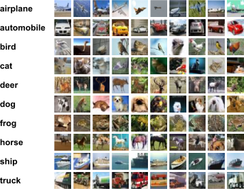
The CIFAR-10 and CIFAR-100 are labeled subsets of the 80 million tiny images dataset. They were collected by Alex Krizhevsky, Vinod Nair, and Geoffrey Hinton.
The CIFAR-10 dataset consists of 60000 32x32 colour images in 10 classes, with 6000 images per class. There are 50000 training images and 10000 test images.
ImageNet
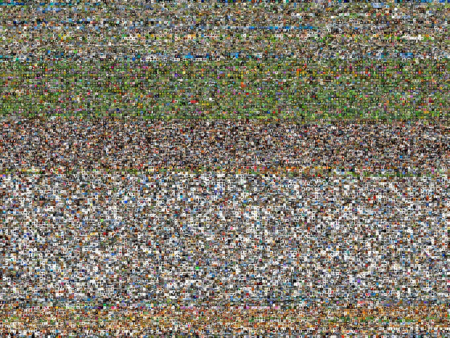
- The ImageNet project is a large visual database designed for use in visual object recognition software research
Applications
Image classifcation
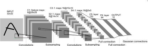
- Architecture of LeNet-5 a Convolutional Neural Network, here for digit recognition, but is extended to character recognition.
Games
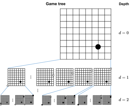
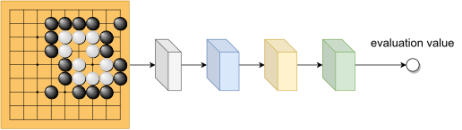
- Go game