8 PROBABILISTIC REASONING OVER TIME
8.1 Temporal Probabilistic Model
Temporal Probabilistic Model
Temporal Probabilistic Model
Why do we need temporal probabilistic model?
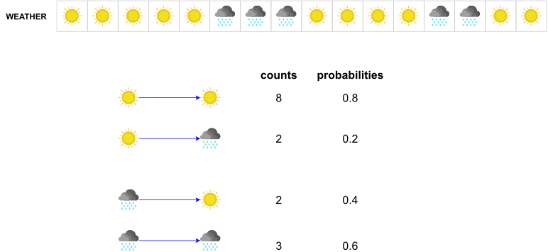
The world changes over time (random process), and what happens now impacts what will happen in the future. We need to track and predict it
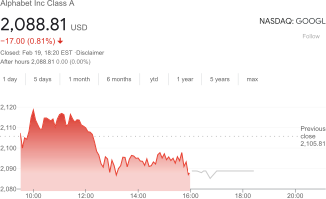
Stock market
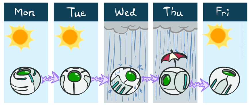
Weather
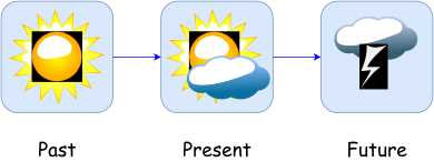
How to model the time?
- View the world as time slices: discrete time steps; step size depends on problem
State variables \boldsymbol{X}_{t} (often hidden): set of unobservable state variables at time t
State of the environment
Not directly observable but defines causal dynamics
Evidence variables \boldsymbol{E}_{t}: set of observable evidence variables at time t
- Caused by the state of the environment
- Notation: \boldsymbol{X}_{a:b}=\boldsymbol{X}_{a},\boldsymbol{X}_{a+1},\ldots,\boldsymbol{X}_{b-1},\boldsymbol{X}_{b}
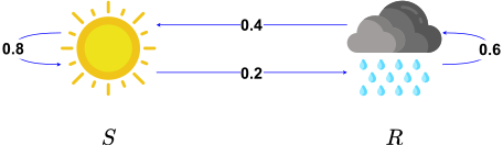
Transition model: How the world evolves \begin{equation} P(\boldsymbol{X}_{t}\mid\boldsymbol{X}_{0:t-1}) \end{equation}
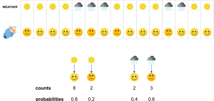
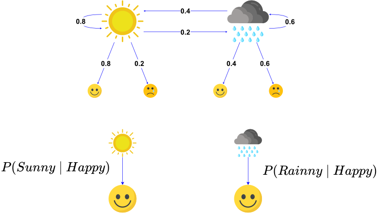
Sensor/observation model: How the evidence variables get their values \begin{equation} P(\boldsymbol{E}_{t}\mid\boldsymbol{X}_{0:t},\boldsymbol{E}_{0:t-1}) \end{equation}
Markov process
Markov process
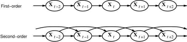
Markov process is a random process with Markov assumption “\boldsymbol{X}_{t} depends on bounded subset of \boldsymbol{X}_{0:t-1}”
First-order Markov process: \begin{equation} P(\boldsymbol{X}_{t}\mid\boldsymbol{X}_{0:t-1})=P(\boldsymbol{X}_{t}\mid\boldsymbol{X}_{t-1}) \end{equation}
Second-order Markov process: \begin{equation} P(\boldsymbol{X}_{t}\mid\boldsymbol{X}_{0:t-1})=P(\boldsymbol{X}_{t}\mid\boldsymbol{X}_{t-2},\boldsymbol{X}_{t-1}) \end{equation}
Sensor Markov assumption: \begin{equation} P(\boldsymbol{E}_{t}\mid\boldsymbol{X}_{0:t},\boldsymbol{E}_{0:t-1})=P(\boldsymbol{E}_{t}\mid\boldsymbol{X}_{t}) \end{equation}
Stationary process:
transition model P(\boldsymbol{X}_{t}\mid\boldsymbol{X}_{t-1}) fixed for all t
sensor model P(\boldsymbol{E}_{t}\mid\boldsymbol{X}_{t}) fixed for all t
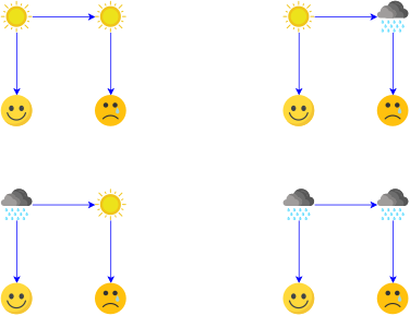
Example
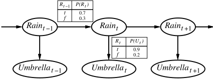
First-order Markov assumption may not be exactly true in real world!
Possible fixes:
Increase order of Markov process
Augment state, e.g., add Temp_{t}, Pressure_{t}
8.2 Inference in Temporal Models
Inference tasks
Filtering: computing the belief state, the posterior distribution over the most recent state given all evidence to date P(X_{t}\mid e_{1:t})
Prediction: computing the posterior distribution over the future state, given all evidence to date P(X_{t+k}\mid e_{1:t})\text{ for }k>0
Smoothing: computing the posterior distribution over a past state, given all evidence up to the present. P(X_{k}\mid e_{1:t})\text{ for }0\leq k<t
Most likely explanation: given a sequence of observations, find the sequence of states that is most likely to have generated those observations \arg\max_{x_{1:t}}P(x_{1:t}\mid e_{1:t})
Filtering
Filtering
Given the result of filtering up to time t, we needs to compute the result for t+1 from the new evidence e_{t+1}, \begin{align} P(X_{t+1}\mid e_{1:t+1}) & = & P(X_{t+1}\mid e_{1:t},e_{t+1})\\ & = & \alpha P(e_{t+1}\mid X_{t+1},e_{1:t})P(X_{t+1}\mid e_{1:t})\\ & = & \alpha P(e_{t+1}\mid X_{t+1})P(X_{t+1}\mid e_{1:t}) \end{align}
We obtain the one-step prediction for the next state by conditioning on the current state X_{t}: \begin{align} P(X_{t+1}\mid e_{1:t+1}) & = & \alpha P(e_{t+1}\mid X_{t+1})\sum_{x_{t}}P(X_{t+1}\mid x_{t},e_{1:t})P(x_{t}\mid e_{1:t})\nonumber \\ & = & \alpha P(e_{t+1}\mid X_{t+1})\sum_{x_{t}}P(X_{t+1}\mid x_{t})P(x_{t}\mid e_{1:t}) \end{align}
The process is given by
f_{1:t+1}=\text{Forward}(f_{1:t},e_{t+1}) where f_{1:t}=P(X_{t}\mid e_{1:t})
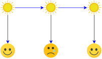
Filtering example
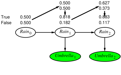
Smoothing
Smoothing
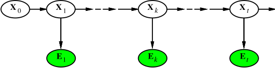
Divide evidence e_{1:t} into e_{1:k}, e_{k+1:t}: \begin{align} P(X_{k}\mid e_{1:t}) & = & P(X_{k}\mid e_{1:k},e_{k+1:t})\nonumber \\ & = & \alpha P(X_{k}\mid e_{1:k})P(e_{k+1:t}\mid X_{k},e_{1:k})\nonumber \\ & = & \alpha P(X_{k}\mid e_{1:k})P(e_{k+1:t}\mid X_{k})\nonumber \\ & = & \alpha f_{1:k}b_{k+1:t} \end{align}
Backward message computed by a backwards recursion: \begin{align} P(e_{k+1:t}\mid X_{k}) & = & \sum_{x_{k+1}}P(e_{k+1:t}\mid X_{k},x_{k+1})P(x_{k+1}\mid X_{k})\nonumber \\ & = & \sum_{x_{k+1}}P(e_{k+1:t}\mid x_{k+1})P(x_{k+1}\mid X_{k})\nonumber \\ & = & \sum_{x_{k+1}}P(e_{k+1}\mid x_{k+1})P(e_{k+2:t}\mid x_{k+1})P(x_{k+1}\mid X_{k}) \end{align}
The process is given by
b_{k+1:t}=\text{Backward}(b_{k+2:t},e_{t+1}) where b_{k+1:t}=P(e_{k+1:t}\mid X_{k})
Smoothing example
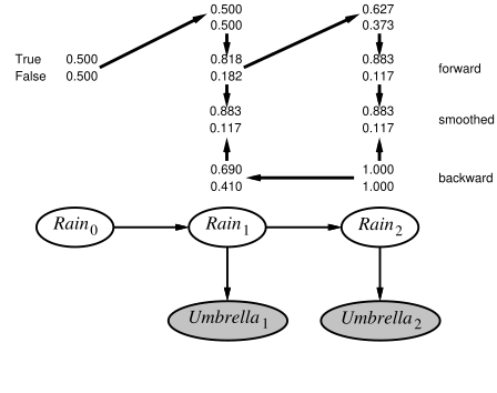
Forward–backward algorithm: cache forward messages along the way
Time linear in t (polytree inference), space O(t\left|f\right|)
Most likely explanation
Most likely explanation
Most likely sequence \neq sequence of most likely states!
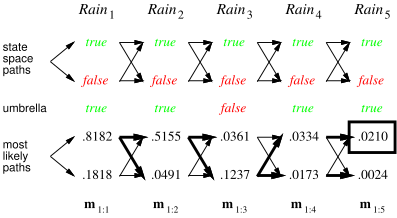
Most likely path to each x_{t+1} = most likely path to some x_{t} plus one more step
\begin{aligned} & \max P(x_{1},\ldots,x_{t},X_{t+1}\mid e_{1:t+1})\\ & =P(e_{t+1}\mid X_{t+1})\max_{x_{t}}\left(P(X_{t+1}\mid x_{t})\max_{x_{1}\ldots x_{t-1}}P(x_{1},\ldots,x_{t-1},x_{t}\mid e_{1:t})\right) \end{aligned}
Identical to filtering, except f_{1:t} replaced by m_{1:t}=\max_{x_{1}\ldots x_{t-1}}P(x_{1},\ldots,x_{t-1},X_{t}\mid e_{1:t}), I.e., m_{1:t}(i) gives the probability of the most likely path to state i.
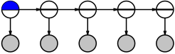
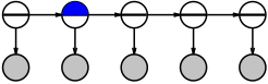
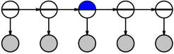
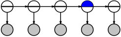
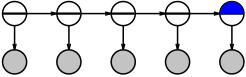
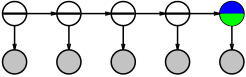
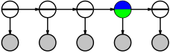
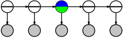
Update has sum replaced by max, giving the Viterbi algorithm: m_{1:t+1}=P(e_{t+1}\mid X_{t+1})\max_{x_{t}}\left(P(X_{t+1}\mid x_{t})m_{1:t}\right)
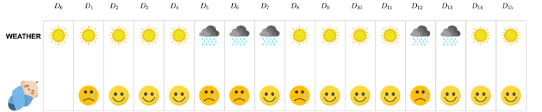
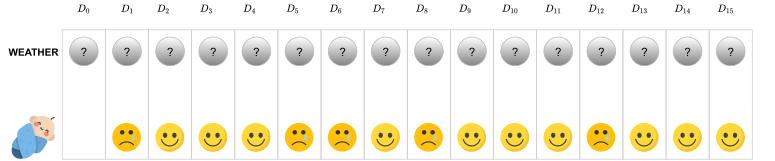
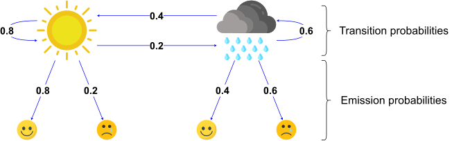
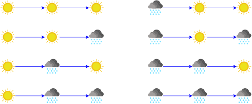
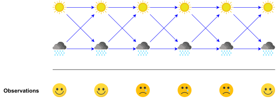
Viterbi example

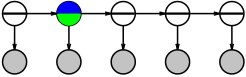
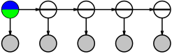
8.4 Kalman Filters
Kalman filters
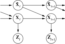
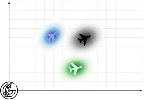
Kalman Filter is a temporal probabilistic model that represents systems described by a set of continuous variables with assumptions: Gaussian prior, linear Gaussian transition model and sensor model
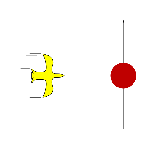
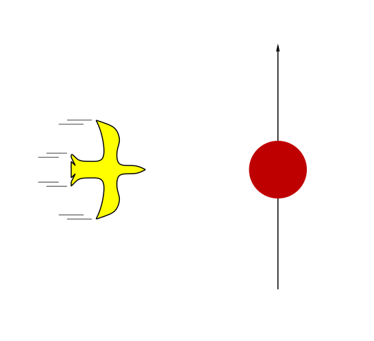
- Tracking a bird flying \boldsymbol{X}_{t}=(position,velocity)=\left(x,y,z,\dot{x},\dot{y},\dot{z}\right)
Updating Gaussian distributions
Prediction step:
If P(X_{t}\mid e_{1:t}) is Gaussian and the transition model P(X_{t+1}\mid x_{t}) is linear Gaussian, then prediction P(X_{t+1}\mid e_{1:t})=\int_{x_{t}}P(X_{t+1}\mid x_{t})P(x_{t}\mid e_{1:t})\,dx_{t} is Gaussian.
If P(X_{t+1}\mid e_{1:t}) is Gaussian and the sensor model P(e_{t+1}|X_{t+1}) is linear Gaussian, then the updated distribution P(X_{t+1}\mid e_{1:t+1})=\alpha P(e_{t+1}\mid X_{t+1})P(X_{t+1}\mid e_{1:t}) is Gaussian
Hence P(X_{t}\mid e_{1:t}) is multivariate Gaussian \mathcal{N}(\boldsymbol{\mu}_{t},\Sigma_{t}) for all t
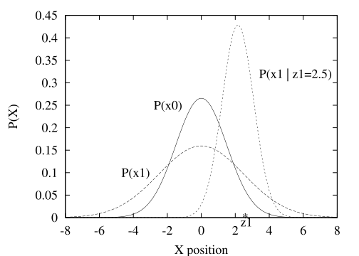
Simple 1-D example
- Gaussian random walk on X–axis, transition s.d. \sigma_{x}, sensor s.d. \sigma_{z} \begin{align*} \mu_{t+1} & =\frac{(\sigma_{t}^{2}+\sigma_{x}^{2})z_{t+1}+\sigma_{z}^{2}\mu_{t}}{\sigma_{t}^{2}+\sigma_{x}^{2}+\sigma_{z}^{2}}\\ \sigma_{t+1}^{2} & =\frac{(\sigma_{t}^{2}+\sigma_{x}^{2})\sigma_{z}^{2}}{\sigma_{t}^{2}+\sigma_{x}^{2}+\sigma_{z}^{2}} \end{align*}
General Kalman update
Transition and sensor models: \begin{equation} \begin{array}{rcl} P(\boldsymbol{x}_{t+1}\mid\boldsymbol{x}_{t}) & = & \mathcal{N}(F\boldsymbol{x}_{t},\Sigma_{x})(\boldsymbol{x}_{t+1})\\ P(\boldsymbol{z}_{t}\mid\boldsymbol{x}_{t}) & = & \mathcal{N}(H\boldsymbol{x}_{t},\Sigma_{z})(\boldsymbol{z}_{t}) \end{array} \end{equation}
F is the matrix for the transition; \Sigma_{x} the transition noise covariance
H is the matrix for the sensors; \Sigma_{z} the sensor noise covariance
Filter computes the following update: \begin{equation} \begin{array}{rcl} \boldsymbol{\mu}_{t+1} & = & F\boldsymbol{\mu}_{t}+K_{t+1}(\boldsymbol{z}_{t+1}-HF\boldsymbol{\mu}_{t})\\ \Sigma_{t+1} & = & (I-K_{t+1})(F\Sigma_{t}F^{\intercal}+\Sigma_{x}) \end{array} \end{equation} where K_{t+1}=(F\Sigma_{t}F^{\intercal}+\Sigma_{x})H^{\intercal}(H(F\Sigma_{t}F^{\intercal}+\Sigma_{x})H^{\intercal}+\Sigma_{z})^{-1} is the Kalman gain matrix
\Sigma_{t} and K_{t} are independent of observation sequence, so compute offline
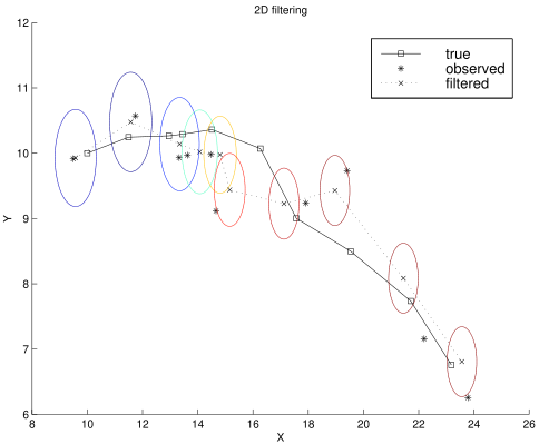
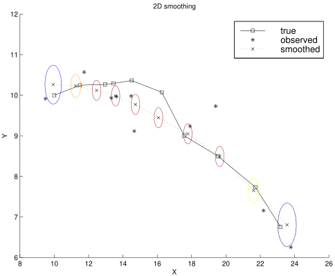
2-D tracking example
2-D tracking example: filtering
2-D tracking example: smoothing
Where it breaks
Cannot be applied if the transition model is nonlinear
Extended Kalman Filter models transition as locally linear around x_{t}=\boldsymbol{\mu}_{t}
- Fails if systems is locally unsmooth
8.5 Dynamic Bayesian Networks
Dynamic Bayesian networks
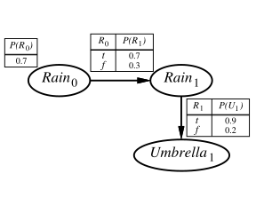
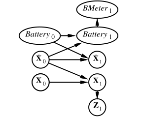
X_{t}, E_{t} contain arbitrarily many variables in a replicated Bayes net
DBNs vs. HMMs
Every HMM is a single-variable DBN; every discrete DBN is an HMM
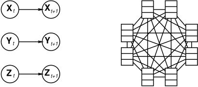
Sparse dependencies \Rightarrow exponentially fewer parameters;
e.g., 20 state variables, three parents each
DBN has 20\times2^{3}=160 parameters, HMM has 2^{20}\times2^{20}\approx10^{12}
DBNs vs Kalman filters
Every Kalman filter model is a DBN, but few DBNs are KFs; real world requires non-Gaussian posteriors
E.g., where are bin Laden and my keys? What’s the battery charge?
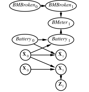
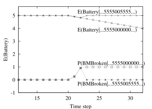
Exact inference in DBNs
Naive method: unroll the network and run any exact algorithm

Problem: inference cost for each update grows with t
Rollup filtering: add slice t+1, “sum out” slice t using variable elimination
Largest factor is O(d^{n+1}), update cost O(d^{n+2}) (cf. HMM update cost O(d^{2n}))
Likelihood weighting for DBNs
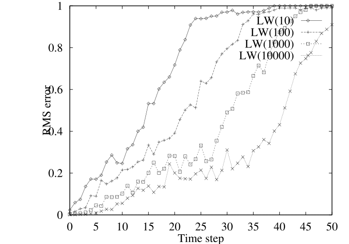
Set of weighted samples approximates the belief state

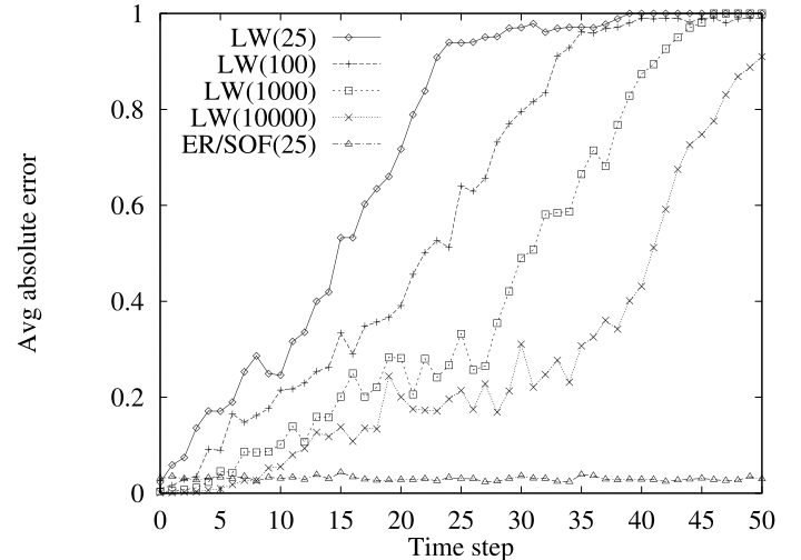
LW samples pay no attention to the evidence!
\Rightarrow fraction “agreeing” falls exponentially with t
\Rightarrow number of samples required grows exponentially with t
Particle Filtering
Particle filtering
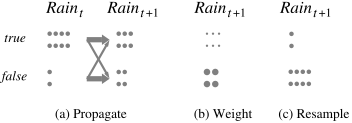
Particle filtering is a model to focus on the population of samples (“particles”) that tracks the high-likelihood regions of the state-space
Widely used for tracking nonlinear systems, esp. in vision
Also used for simultaneous localization and mapping in mobile robots 10^{5}-dimensional state space
Filter task
Writing N(\boldsymbol{x}_{t}\mid\boldsymbol{e}_{1:t}) for the number of samples occupying state \boldsymbol{x}_{t} after observations \boldsymbol{e}_{1:t} have been processed. Assume consistent at time t: \begin{equation} N(\boldsymbol{x}_{t}\mid\boldsymbol{e}_{1:t})/N=P(\boldsymbol{x}_{t}\mid\boldsymbol{e}_{1:t}) \end{equation}
Propagate forward populations of \boldsymbol{x}_{t+1}: \begin{equation} N(\boldsymbol{x}_{t+1}\mid\boldsymbol{e}_{1:t})=\sum_{x_{t}}P(\boldsymbol{x}_{t+1}\mid\boldsymbol{x}_{t})N(\boldsymbol{x}_{t}\mid\boldsymbol{e}_{1:t}) \end{equation}
Weight samples by their likelihood for \boldsymbol{e}_{t+1}: \begin{equation} W(\boldsymbol{x}_{t+1}\mid\boldsymbol{e}_{1:t+1})=P(\boldsymbol{e}_{t+1}\mid\boldsymbol{x}_{t+1})N(\boldsymbol{x}_{t+1}\mid\boldsymbol{e}_{1:t}) \end{equation}
Resample to obtain populations proportional to W: \begin{align} N(\boldsymbol{x}_{t+1}\mid\boldsymbol{e}_{1:t+1})/N & = & \alpha W(\boldsymbol{x}_{t+1}\mid\boldsymbol{e}_{1:t+1})\nonumber \\ & = & \alpha P(\boldsymbol{e}_{t+1}\mid\boldsymbol{x}_{t+1})N(\boldsymbol{x}_{t+1}\mid\boldsymbol{e}_{1:t})\nonumber \\ & = & \alpha P(\boldsymbol{e}_{t+1}\mid\boldsymbol{x}_{t+1})\sum_{x_{t}}P(\boldsymbol{x}_{t+1}\mid x_{t})N(\boldsymbol{x}_{t}\mid\boldsymbol{e}_{1:t})\nonumber \\ & = & \alpha P(\boldsymbol{e}_{t+1}\mid\boldsymbol{x}_{t+1})\sum_{x_{t}}P(\boldsymbol{x}_{t+1}\mid\boldsymbol{x}_{t})P(\boldsymbol{x}_{t}\mid\boldsymbol{e}_{1:t})\nonumber \\ & = & P(\boldsymbol{x}_{t+1}\mid\boldsymbol{e}_{1:t+1}) \end{align}
Particle filtering performance
- Approximation error of particle filtering remains bounded over time, at least empirically—theoretical analysis is difficult
8.6 Keeping Track of Many Objects
Summary
Temporal models use state and sensor variables replicated over time
Markov assumptions and stationarity assumption, so we need
transition model P(X_{t}\mid X_{t-1})
sensor model P(E_{t}\mid X_{t})
Tasks are filtering, prediction, smoothing, most likely sequence; all done recursively with constant cost per time step
Hidden Markov models have a single discrete state variable; used for speech recognition
Kalman filters allow n state variables, linear Gaussian, O(n^{3}) update
Dynamic Bayes nets subsume HMMs, Kalman filters; exact update intractable
Particle filtering is a good approximate filtering algorithm for DBNs