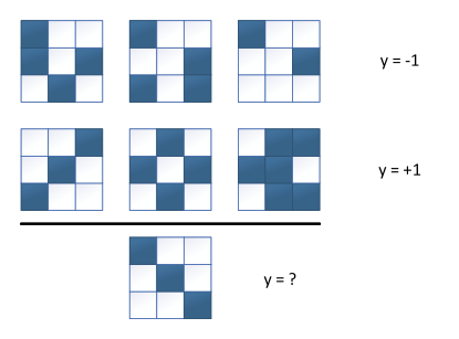
4 DECISION TREE MODEL

Learning diagram

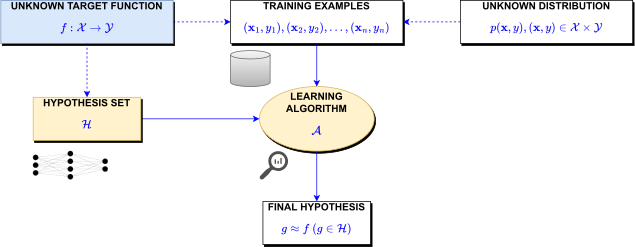
4.1 Decision Tree Representation

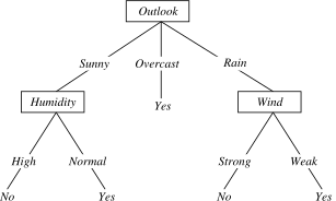
Decision tree representation

Each internal node tests an attribute
Each branch corresponds to attribute value

Each leaf node assigns a classification

Day	Outlook	Temperature	Humidity	Wind	PlayTennis?
D1	Sunny	Hot	High	Weak	No \ominus
D2	Sunny	Hot	High	Strong	No \ominus
D3	Overcast	Hot	High	Weak	Yes \oplus
D4	Rain	Mild	High	Weak	Yes \oplus
D5	Rain	Cool	Normal	Weak	Yes \oplus
...	...	...	...	...	...

When to Consider Decision Trees

Classification problems
Instances describable by attribute–value pairs
Attributes are discrete valued
Target function is discrete valued

Problem Statement

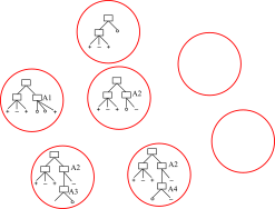
Hypothesis set \mathcal{H} (finite set, there are 2^{2^{n}} trees for n binary attributes and binary target)
- With 6 binary attributes, there are 18,446,744,073,709,551,616 trees
Task T: to predict y from \boldsymbol{x} by outputting \hat{y}=h_{T}(\mathbf{x})=T(\boldsymbol{x})
Performance measure P: classification error

4.2 Learning Algorithm

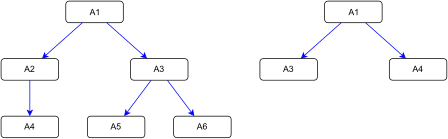
Which tree is best?

Which tree would be chosen? if both trees are fitted to \mathcal{D}=\{(\boldsymbol{x}_{1},y_{1})...(\boldsymbol{x}_{N},y_{N})\}

Occam’s Razor

Principle of Occam’s Razor The simplest model that fits the data is also the most plausible (prefer the shortest hypothesis that fits the data)

Inductive Bias: Preference for short trees, and for those with high information gain attributes near the root

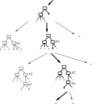
Top-Down Algorithm

function Decision-Tree-Learning(examples, attributes)

if all examples have the same classification then return the classification

else if attributes is \emptyset then return Plurality-Value(examples)

else

A\leftarrow the “best” decision attribute for next node

Assign A as decision attribute for node

For each value of A, create new descendant of node

Split training examples to child nodes and repeat these steps

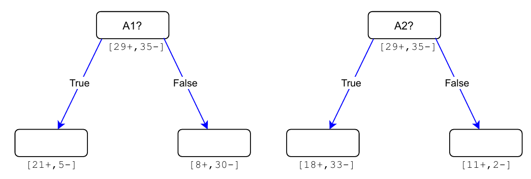
Which attribute is best?

Big Picture

Entropy

Information Gain

S is a sample of training examples
p_{\oplus} is the proportion of positive examples in S
p_{\ominus} is the proportion of negative examples in S

Entropy measures the impurity of S \begin{equation} Entropy(S)=-\left(p_{\oplus}\log_{2}p_{\oplus}+p_{\ominus}\log_{2}p_{\ominus}\right) \end{equation}

S is a set of items with C classes, and let \boldsymbol{p}=\{p_{i}\}_{i=1}^{C} be the fraction of items labeled with class i in the set.

Entropy measures the impurity of S \begin{equation} Entropy(S)=-\sum_{i=1}^{C}p_{i}\log_{2}p_{i} \end{equation}

Average entropy on attribute A \begin{equation} AE(S,A)=\sum_{v\in Values(A)}\frac{|S_{v}|}{|S|}Entropy(S_{v}) \end{equation}
Information gain is expected reduction in entropy on A \begin{equation} Gain(S,A)=Entropy(S)-AE(S,A) \end{equation}
The best attribute is an attribute that has the highest information gain

Gini

Gini index

Gini impurity for a set of items S with C classes, and let \boldsymbol{p}=\{p_{i}\}_{i=1}^{C} be the fraction of items labeled with class i in the set. \begin{equation} GiniImp(S)=1-\sum_{i=1}^{C}p_{i}^{2} \end{equation}
Gini index on attribute A \begin{equation} GiniIndex(S,A)=\sum_{v\in Values(A)}\frac{|S_{v}|}{|S|}GiniImp(S_{v}) \end{equation}

Misclassification

Misclassification index

Misclassification impurity index for a set of items S with C classes, and let \boldsymbol{p}=\{p_{i}\}_{i=1}^{C} be the fraction of items labeled with class i in the set. \begin{equation} MisImp(S)=1-\max\left\{ p_{i}\right\} _{i=1}^{C} \end{equation}
Misclassification index on attribute A \begin{equation} MisIndex(S,A)=\sum_{v\in Values(A)}\frac{|S_{v}|}{|S|}MisImp(S_{v}) \end{equation}

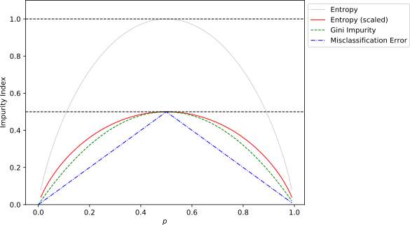
Entropy, Gini and Misclassification

Example 1

Find decision tree T given the following training data

Day	Outlook	Temperature	Humidity	Wind	PlayTennis?
D1	Sunny	Hot	High	Weak	No
D2	Sunny	Hot	High	Strong	No
D3	Overcast	Hot	High	Weak	Yes
D4	Rain	Mild	High	Weak	Yes
D5	Rain	Cool	Normal	Weak	Yes
D6	Rain	Cool	Normal	Strong	No
D7	Overcast	Cool	Normal	Strong	Yes
D8	Sunny	Mild	High	Weak	No
D9	Sunny	Cool	Normal	Weak	Yes
D10	Rain	Mild	Normal	Weak	Yes
D11	Sunny	Mild	Normal	Strong	Yes
D12	Overcast	Mild	High	Strong	Yes
D13	Overcast	Hot	Normal	Weak	Yes
D14	Rain	Mild	High	Strong	No

Example 1 - Finding Decision Tree and Converting to Rules

IF	(Outlook=Sunny)\land(Humidity=High)	THEN	PlayTennis=No
ELIF	(Outlook=Sunny)\land(Humidity=Normal)	THEN	PlayTennis=Yes
ELIF	Outlook=Overcast	THEN	PlayTennis=Yes
ELIF	(Outlook=Rain)\land(Wind=Strong)	THEN	PlayTennis=No
ELIF	(Outlook=Rain)\land(Wind=Weak)	THEN	PlayTennis=Yes
ELIF		THEN	failure

Evaluating Association Rules

An association rule is an implication of the form X\to Y or IF X THEN Y

Support of the association rule \begin{equation} \text{support}(X,Y)=P(X,Y)=\frac{\text{\#count}(X,Y)}{\text{total samples}} \end{equation}
Confidence of the association rule \begin{equation} \text{confidence}(X\to Y)=P(Y\mid X)=\frac{\text{\#count}(X,Y)}{\text{\#count}(X)} \end{equation}

Example 2

Find decision tree T given the following training data

#	Input attributes										Goal
	Alt	Bar	Fri	Hun	Pat	Price	Rain	Res	Type	Est	Will Wait
1	Yes	No	No	Yes	Some	$$$	No	Yes	French	0–10	T
2	Yes	No	No	Yes	Full	$	No	No	Thai	30–60	F
3	No	Yes	No	No	Some	$	No	No	Burger	0–10	T
4	Yes	No	Yes	Yes	Full	$	Yes	No	Thai	10–30	T
5	Yes	No	Yes	No	Full	$$$	No	Yes	French	>60	F
6	No	Yes	No	Yes	Some	$$	Yes	Yes	Italian	0–10	T
7	No	Yes	No	No	None	$	Yes	No	Burger	0–10	F
8	No	No	No	Yes	Some	$$	Yes	Yes	Thai	0–10	T
9	No	Yes	Yes	No	Full	$	Yes	No	Burger	>60	F
10	Yes	Yes	Yes	Yes	Full	$$$	No	Yes	Italian	10–30	F
11	No	No	No	No	None	$	No	No	Thai	0–10	F
12	Yes	Yes	Yes	Yes	Full	$	No	No	Burger	30–60	T

Example 2 - Finding Decision Tree

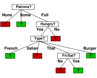
Word Example

Find decision tree T given the following training datasets

Find all stumps (decision tree with one node)

#	Vị	Màu	Vỏ	Độc tính
1	Ngọt	Đỏ	Nhẵn	Không
2	Cay	Đỏ	Nhẵn	Có
3	Chua	Vàng	Có gai	Không
4	Cay	Vàng	Có gai	Có
5	Ngọt	Tím	Có gai	Không
6	Chua	Vàng	Nhẵn	Không
7	Ngọt	Tím	Nhẵn	Không
8	Cay	Tím	Có gai	Có
9	Cay	Tím	Có gai	Không
10	Cay	Tím	Có gai	Có
11	Cay	Vàng	Có gai	Có

4.3 Generalization And Overfitting

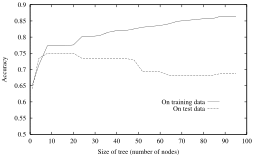
Overfitting in Decision Tree Learning

Avoiding Overfitting

How can we avoid overfitting?

stop growing when data split not statistically significant
grow full tree, then post-prune

How to select “best” tree:

Measure performance over training data
Measure performance over separate validation data set
Minimize error(tree)+{\color{green}\lambda}size(tree)

4.4 Continuous Valued Attributes

Continuous Valued Attributes

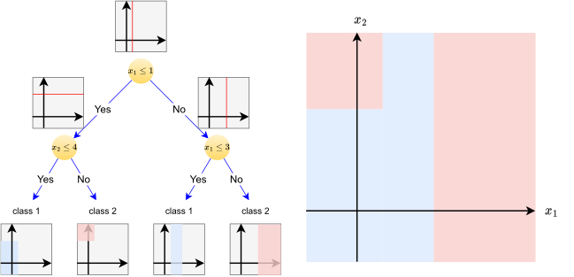
Create a discrete attribute for continuous variable

Binary node

Temperature>36 or Temperature\leq36
General node

Temperature\in\{(-\infty,0],(0,10],(10,20],(20,\infty)\}

Decision Tree with Continuous Valued Attributes

Extended Top-Down Algorithm

procedure GenerateTree(\mathcal{D})

if Entropy(\mathcal{D}) < \epsilon

Create leaf labelled by majority class in \mathcal{D}

return

i \gets SplitAttribute(\mathcal{D})

for each branch of X_{i}

Find \mathcal{D}_{i} falling in branch

GenerateTree(\mathcal{D}_{i})

function SplitAttribute(\mathcal{D})

entropy_{min} \gets \infty

for all attributes X_{i} where i=1,...,d

if X_{i} is discrete with n values

Split \mathcal{D} into \mathcal{D}_{1},...,\mathcal{D}_{n} by X_{i}

e \gets AverageEntropy(\mathcal{D}_{1},...,\mathcal{D}_{n})

if e<entropy_{min}: entropy_{min}\gets e, i_{min} \gets i

if X_{i} is numeric

for all possible splits

Split \mathcal{D} into \mathcal{D}_{1},\mathcal{D}_{2} on X_{i}

e \gets AverageEntropy(\mathcal{D}_{1},\mathcal{D}_{2})

if e<entropy_{min}: entropy_{min}\gets e, i_{min}\gets i

return i_{min}

Example 3

Find decision tree T given the following training data

Day	Outlook	Temperature	Humidity	Wind	PlayTennis?
D1	Sunny	37	High	Weak	No
D2	Sunny	37	High	Strong	No
D3	Overcast	38	High	Weak	Yes
D4	Rain	28	High	Weak	Yes
D5	Rain	20	Normal	Weak	Yes
D6	Rain	18	Normal	Strong	No
D7	Overcast	19	Normal	Strong	Yes
D8	Sunny	27	High	Weak	No
D9	Sunny	21	Normal	Weak	Yes
D10	Rain	26	Normal	Weak	Yes
D11	Sunny	26	Normal	Strong	Yes
D12	Overcast	27	High	Strong	Yes
D13	Overcast	36	Normal	Weak	Yes
D14	Rain	28	High	Strong	No

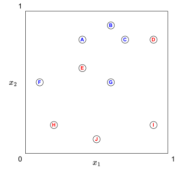
Example 4

Find decision tree T given the following training data

# x_{1} x_{2} label

A 0.4 0.8 1

B 0.6 0.9 1

C 0.7 0.8 1

D 0.9 0.8 -1

E 0.4 0.6 -1

F 0.1 0.5 1

G 0.6 0.5 1

H 0.2 0.2 -1

I 0.9 0.2 -1

J 0.5 0.1 -1

#	x_{1}	x_{2}	label
A	0.4	0.8	1
B	0.6	0.9	1
C	0.7	0.8	1
D	0.9	0.8	-1
E	0.4	0.6	-1
F	0.1	0.5	1
G	0.6	0.5	1
H	0.2	0.2	-1
I	0.9	0.2	-1
J	0.5	0.1	-1

4.5 Regression Trees

Regression Trees

A regression tree is constructed in almost the same manner as a classification tree, except that the impurity measure that is appropriate for classification is replaced by a measure appropriate for regression.

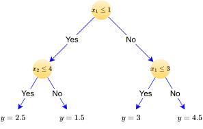
Loss Function

	Classification	Regression
`Dataset`	\mathcal{D}=\{(x_{1,}y_{1}),...,(x_{n},y_{n}\}
`Target`	y_{i} categorical value	y_{i} real value
Loss function	Entropy	Error
		\overline{y}=\frac{1}{n}\sum_{i=1}^{n}y_{i}
		e=\frac{1}{n}\sum(y_{i}-\overline{y})^{2}
		cv=\dfrac{\sqrt{e}}{\overline{y}}

Top-Down Algorithm

procedure GenerateTree(\mathcal{D})

if Error(\mathcal{D}) < \epsilon

Create leaf valued by \overline{y}

return

i \gets SplitAttribute(\mathcal{D})

for each branch of X_{i}

Find \mathcal{D}_{i} falling in branch

GenerateTree(\mathcal{D}_{i})

function SplitAttribute(\mathcal{D})

e_{min} \gets \infty

for all attributes X_{i} where i=1,...,d

if X_{i} is discrete with n values

Split \mathcal{D} into \mathcal{D}_{1},...,\mathcal{D}_{n} by X_{i}

e \gets AverageError(\mathcal{D}_{1},...,\mathcal{D}_{n})

if e<e_{min}: e_{min}\gets e, i_{min} \gets i

if X_{i} is numeric

for all possible splits

Split \mathcal{D} into \mathcal{D}_{1},\mathcal{D}_{2} on X_{i}

e \gets AverageError(\mathcal{D}_{1},\mathcal{D}_{2})

if e<e_{min}: e_{min}\gets e, i_{min}\gets i

return i_{min}

Example 5

Find regression tree T given the following training data

Day	Outlook	Temperature	Humidity	Wind	Play time (m)
D1	Rainy	Hot	High	Weak	26
D2	Rainy	Hot	High	Strong	30
D3	Overcast	Hot	High	Weak	46
D4	Sunny	Mild	High	Weak	46
D5	Sunny	Cool	Normal	Weak	62
D6	Sunny	Cool	Normal	Strong	23
D7	Overcast	Cool	Normal	Strong	43
D8	Rainy	Mild	High	Weak	36
D9	Rainy	Cool	Normal	Weak	38
D10	Sunny	Mild	Normal	Weak	46
D11	Rainy	Mild	Normal	Strong	48
D12	Overcast	Mild	High	Strong	62
D13	Overcast	Hot	Normal	Weak	44
D14	Sunny	Mild	High	Strong	30

4.6 Multivariate Trees

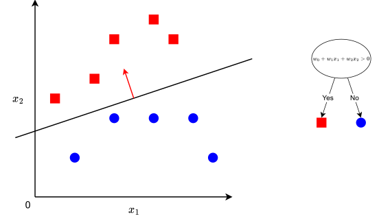
Multivariate Trees

In the case of a univariate tree, only one input dimension is used at a split.
In a multivariate tree, at a decision node, all input dimensions can be used and thus it is more general.

Programming Examples

import matplotlib.pyplot as plt
from sklearn.datasets import load_iris
from sklearn.tree import DecisionTreeClassifier, plot_tree

iris = load_iris()
clf = DecisionTreeClassifier(criterion="entropy")
clf.fit(iris.data, iris.target)
plot_tree(clf, filled=True)
plt.show()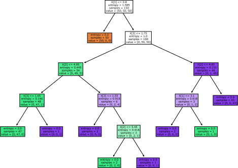

Learning diagram

4.1 Decision Tree Representation

Decision tree representation

When to Consider Decision Trees

Problem Statement

4.2 Learning Algorithm

Which tree is best?

Occam’s Razor

Top-Down Algorithm

Which attribute is best?

Big Picture

Entropy

Information Gain

Gini

Gini index

Misclassification

Misclassification index

Entropy, Gini and Misclassification

Example 1

Example 1 - Finding Decision Tree and Converting to Rules

Evaluating Association Rules

Example 2

Example 2 - Finding Decision Tree

Word Example

4.3 Generalization And Overfitting

Overfitting in Decision Tree Learning

Avoiding Overfitting

4.4 Continuous Valued Attributes

Continuous Valued Attributes

Decision Tree with Continuous Valued Attributes

Extended Top-Down Algorithm

Example 3

Example 4

4.5 Regression Trees

Regression Trees

Loss Function

Top-Down Algorithm

Example 5

4.6 Multivariate Trees

Multivariate Trees

Programming Examples

A Learning Puzzle Revisited

4.7 References