13 NEURAL NETWORKS
Previous Lessons
Ensemble
Uncertainty
Feature representation
Feature transformation
Hidden variables
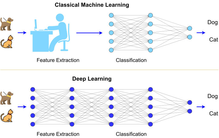
Deep Learning vs. Classical Machine Learning
13.1 Artificial Neural Network
What is a neural network?
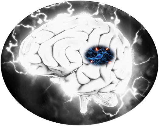
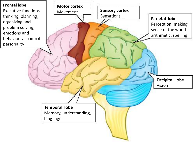
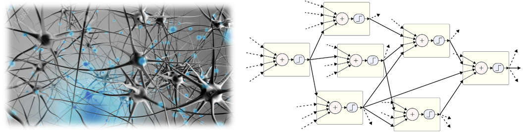
Neural network is a reasoning model based on the human brain, including billions of neurons and trillion connections between them.
The biological brain is considered as a highly complex, nonlinear and parallel information-processing system.
Number of neurons 10^{10}
Connections per neuron 10^{4-5}
Neuron switching time .001 second
Scene recognition time .1 second
Artificial neural networks
Artificial neural networks (ANNs) resembles the human brain in terms of learning mechanisms.
An ANN consists of a number of very simple and highly interconnected processors (or neurons), arranging in a hierarchy of layers.
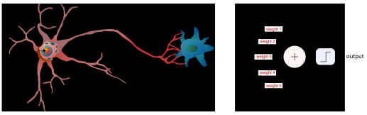
Neuron
Each neuron is an elementary information-processing unit.
The neurons are connected by links passing signals from one neuron to another.
Each neuron receives a number of input signals through its connections and produces at most a single output signal.
Each link associates with a numerical weight expressing the strength of the neuron input \to basic means of long-term memory in ANNs
ANNs “learn” through repeated adjustments of these weights
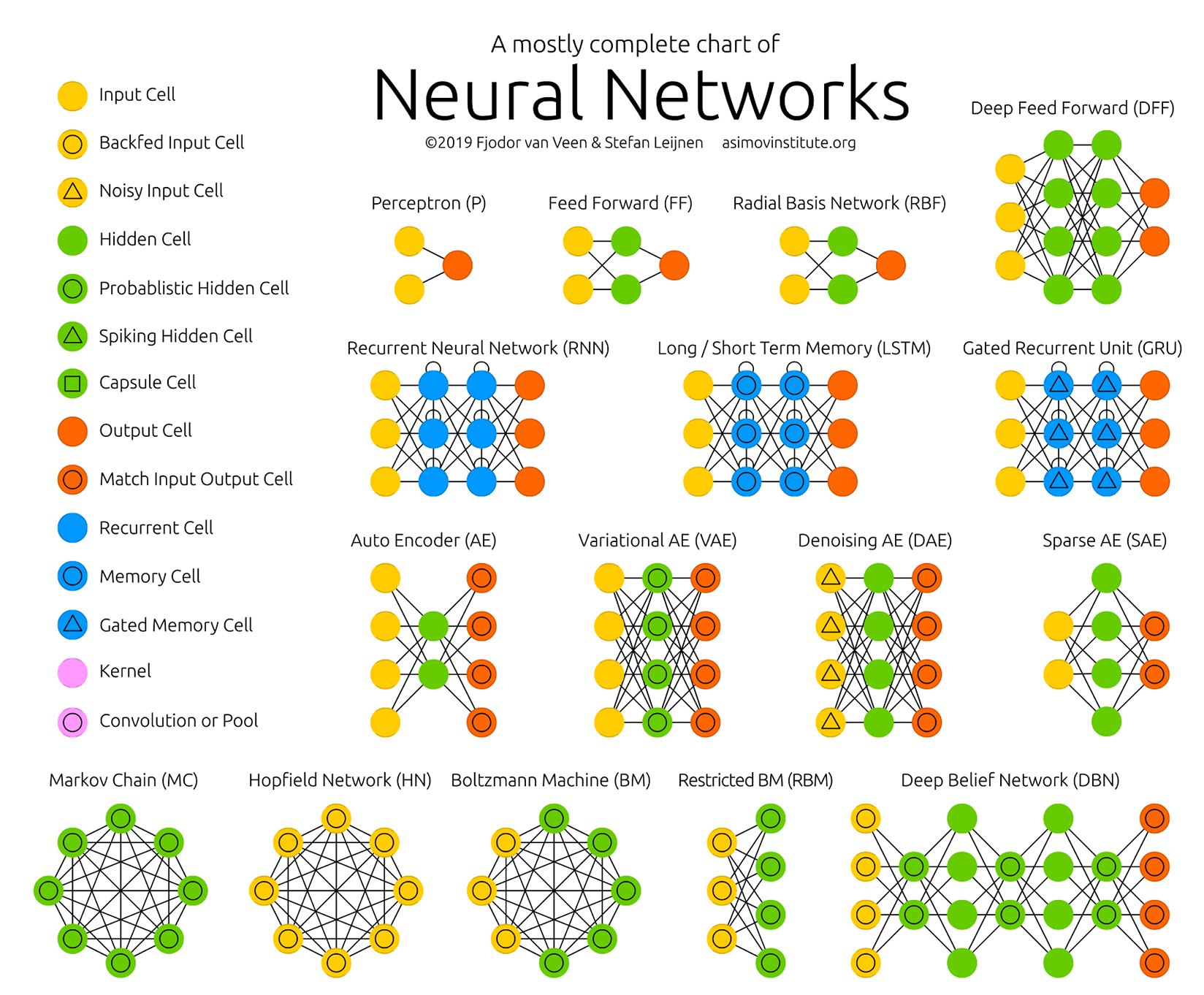
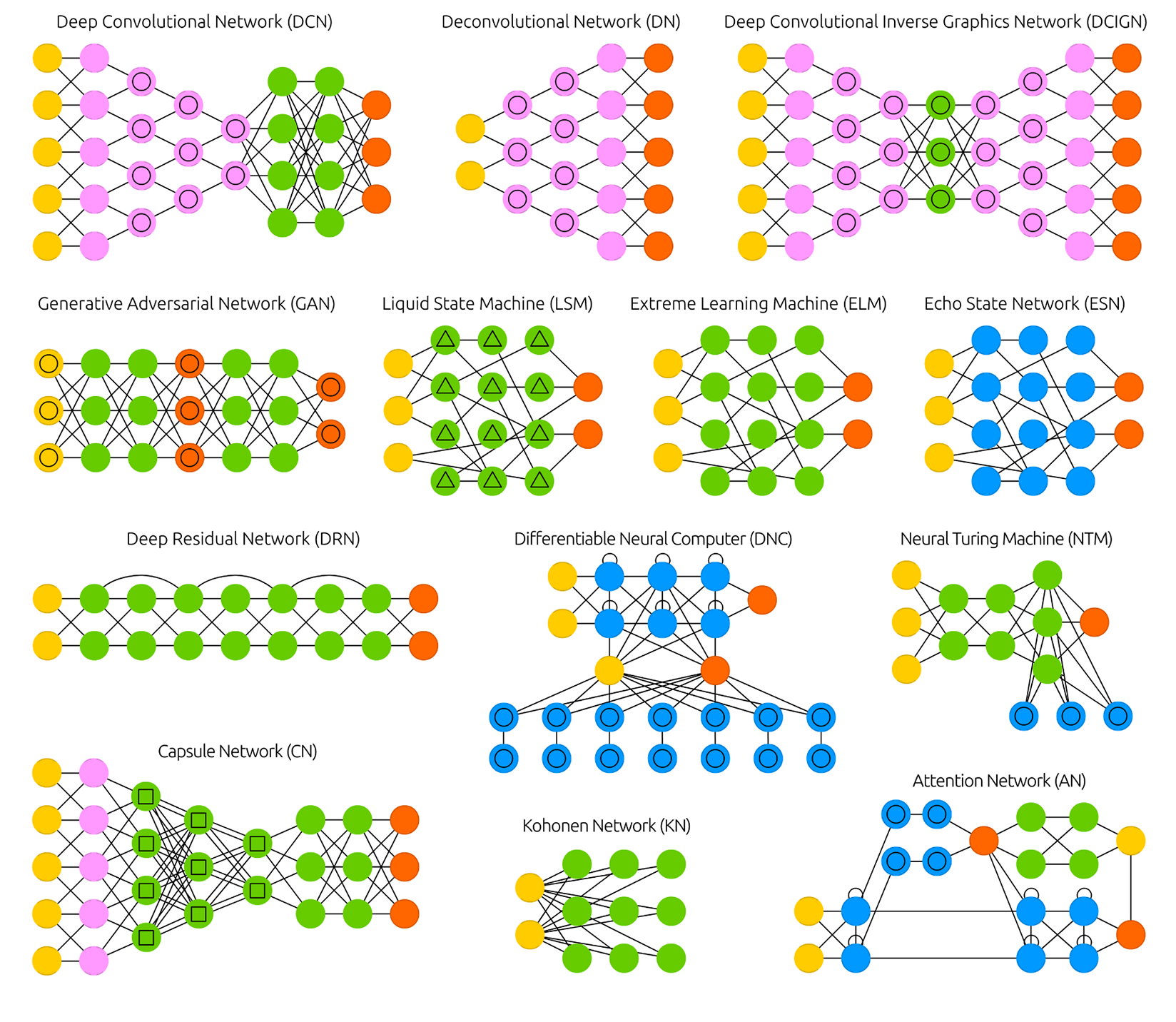
The network architecture
The network architecture includes
How many neurons are to be used?
How the neurons are to be connected to form a network?
Some architectures
13.2 Perceptron: The simplest ANN (Revisited)
Perceptron Model
A perceptron proposed by Minsky-Papert, more general than McCulloch-Pitts neuron, consists of n inputs x_{1},...,x_{n} and 1 output o
First, it computes a weighted sum of its inputs \begin{equation} s=\sum_{i=0}^{n}w_{i}x_{i}=w_{0}+w_{1}x_{1}+\cdots+w_{n}x_{n} \end{equation}
Then it applies an activation function g(s) (sign, sigmoid etc.)
\begin{equation} o(x_{1},\ldots,x_{n}) = g(s) = \left\{ \begin{array}{rl} 1 & \text{if } s \ge 0 \\ -1 & \text{otherwise.} \end{array} \right. \end{equation}

Representation
- Perceptron can represent some useful functions
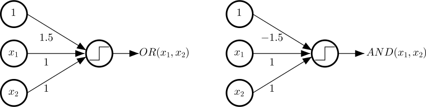
| x_{1} | x_{2} | OR(x_{1},x_{2}) |
|---|---|---|
| -1 | -1 | -1 |
| -1 | 1 | 1 |
| 1 | -1 | 1 |
| 1 | 1 | 1 |
| x_{1} | x_{2} | AND(x_{1},x_{2}) |
|---|---|---|
| -1 | -1 | -1 |
| -1 | 1 | -1 |
| 1 | -1 | -1 |
| 1 | 1 | 1 |
Perceptron cannot represent XOR(x_{1},x_{2})
- Solution is to combine perceptrons \to multilayer perceptrons
13.3 Multilayer Perceptrons (MLP)
Learning Model
Neural Network Playground
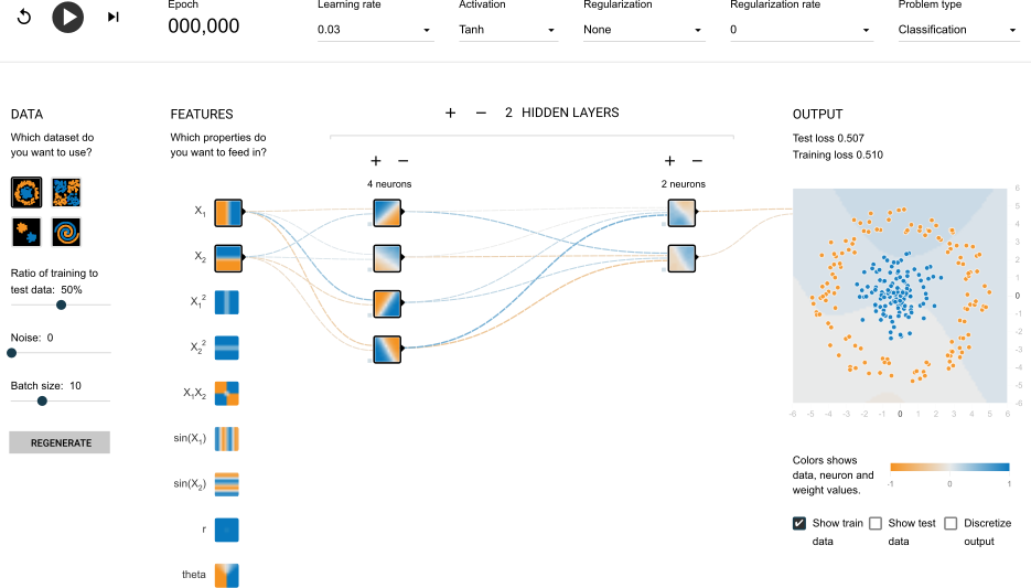
Multilayer Perceptrons
Multilayer perceptrons (neural networks) is a DAG graph that includes many layers.
The first layer is called input layer
The last layer is called output layer
The other are called hidden layers
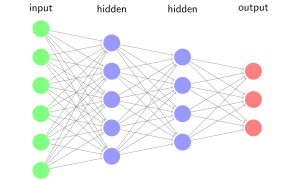
Each layers composed of nodes (neurons)
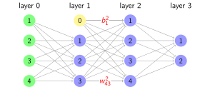
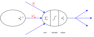
Neurons are connected by directed links to propagate the activation. {\color{red}w_{jk}^{l}} is the weight of the link from the k-th neuron in the (l-1)-th layer to the j-th neuron in the l-th layer
Each layer has weight matrix {\color{red}\boldsymbol{w}^{l}} and a bias vector {\color{red}\boldsymbol{b}^{l}}
- The j-th neuron in the l-th layer has the activation a_{j}^{l}
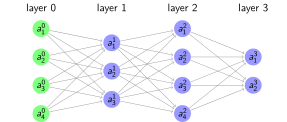
The j-th neuron in the l-th layer first computes a weighted sum of its inputs \begin{equation} in=\sum_{k}{\color{red}w_{jk}^{l}}a_{k}^{l-1}+{\color{red}b_{j}^{l}} \end{equation}
Then it applies an activation function g to this sum to derive the output:
\begin{equation} a_{j}^{l}=g(in)=g\left(\sum_{k}{\color{red}w_{jk}^{l}}a_{k}^{l-1}+{\color{red}b_{j}^{l}}\right)\label{eq} \end{equation}
Activation functions
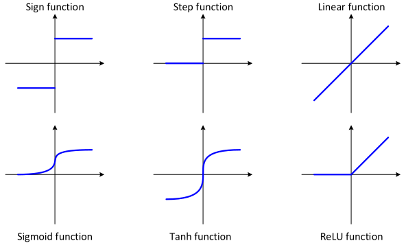
Sign function \begin{equation} a=\text{sign}(x)=\begin{cases} 1 & x\geq0\\ -1 & x<0 \end{cases} \end{equation}
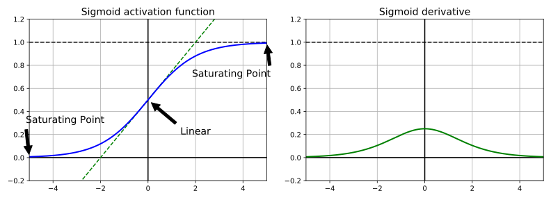
Sigmoid function \begin{equation} a=\sigma(x)=\frac{1}{1+\exp(-x)} \end{equation}
Linear function \begin{equation} a=x \end{equation}
Step function \begin{equation} a=\text{step}(x)=\begin{cases} 1 & x\geq0\\ 0 & x<0 \end{cases} \end{equation}
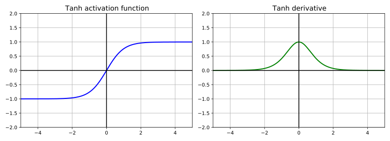
Tanh function \begin{equation} a=\tanh(x)=\frac{e^{x}-e^{-x}}{e^{x}+e^{-x}} \end{equation}
ReLU (rectified linear unit) \begin{equation} a=\text{ReLU}(x)=\begin{cases} x & x\geq0\\ 0 & x<0 \end{cases} \end{equation}
Sigmoid function
Tanh function
Softmax Gate
- The softmax function takes all the network’s outputs and modifies them simultaneously. The result is that the scores are turned into probabilities (this technique is not a normal activation function)
\begin{equation} f_{t}(\boldsymbol{x})=f_{t}(x_{1},x_{2},...,x_{k})=\dfrac{e^{x_{i}}}{\sum_{j=1}^{k}e^{x_{j}}},\text{ for }t=1,...,k \end{equation} \begin{equation} f_{t}(\boldsymbol{x})=f_{t}(x_{1},x_{2},...,x_{k})=\dfrac{e^{x_{i}-M}}{\sum_{j=1}^{k}e^{x_{j}-M}},\text{ stable version} \end{equation} where M=\max(x_{1,}x_{2},...,x_{3})

Universal Approximation Theorem
Expressive Capabilities of MLP
Boolean functions
- Every boolean function can be represented by network with single hidden layer but might require exponential (in number of inputs) hidden units
Continuous functions
Every bounded continuous function can be approximated with arbitrarily small error, by network with one hidden layer
Any function can be approximated to arbitrary accuracy by a network with two hidden layers
Learning Model
Hypothesis set or function space \mathcal{F}=\{f\mid y=f(x;{\color{red}W})\}
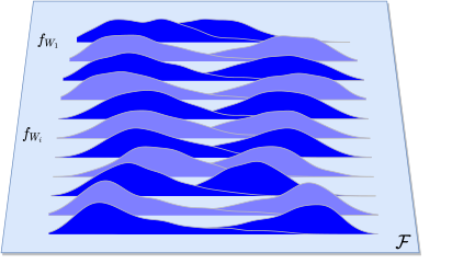
Learning algorithm:
Gradient-based algorithms
Delta learning rule
...
Design Neural Network
Design Neural Network
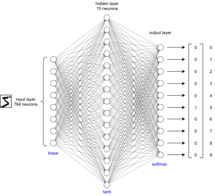
A simple network to classify handwritten digits

The input layer of the network contains neurons encoding the values of the input pixels. Our training data for the network will consist of many 28 by 28 pixel images of scanned handwritten digits, and so the input layer contains 784=28\times28 neurons
The second layer of the network is a hidden layer
The output layer of the network contains 10 neurons. If the first neuron fires, i.e., has an output \approx1, then that will indicate that the network thinks the digit is a 0. If the second neuron fires then that will indicate that the network thinks the digit is a 1. And so on
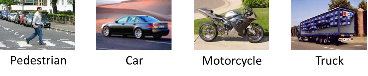
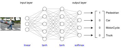
A simple object classification
Neural Network Learning
Neural Network Learning
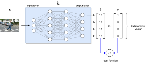
- In training step, we fit the network to the data based on a cost function
Cost Function
In the neural network learning, the selection of output layer depends on the learning problems.
Classification: sigmoid, softmax .etc
Regression: linear etc.
Cost function (lost function) can be derived from many methods, the most common of them
Mean Square Error
Cross Entropy
Let \boldsymbol{y} denotes the desired label of data \boldsymbol{x}, and \tilde{\boldsymbol{y}}=h(\boldsymbol{x}) as the prediction. The cost function C_{MSE} is defined by \begin{equation} C_{MSE}=\frac{1}{k}\sum_{i=1}^{k}(y_{i}-\tilde{y}_{i})^{2} \end{equation}
The cost function defined by Cross Entropy is \begin{equation} C_{CE}=\sum_{i=1}^{k}y_{i}\ln\tilde{y}_{i} \end{equation}
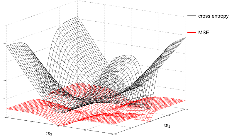
Cross Entropy vs. MSE
Output Types
| Output Type | Output Distribution | Output Layer | Cost Function |
|---|---|---|---|
| Binary | Bernoulli | Sigmoid | Binary cross-entropy |
| Discrete | Multinoulli | Softmax | Discrete cross-entropy |
| Continuous | Gaussian | Linear | Gaussian cross-entropy (MSE) |
| Continuous | Mixture of Gaussian | Mixture Density | Cross-entropy |
Regularization
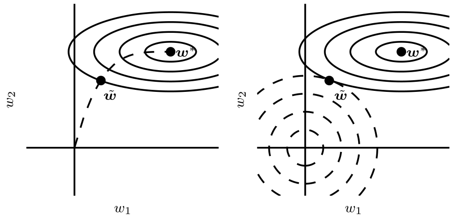
“Regularization is any modification we make to a learning model that is intended to reduce its generalization error but not its training error.”
- To avoid overfitting, we can use the regularized cost function (weight decay) \begin{equation} C_{reg}(\boldsymbol{{\color{red}w}})=C(\boldsymbol{{\color{red}w}})+{\color{green}\lambda}regularizer(\boldsymbol{{\color{red}w}}) \end{equation} where {\color{green}\lambda} is the regularization coefficient (hyper-parameter) that controls the relative importance of the data-dependent error C(\boldsymbol{{\color{red}w}}) and the regularization term \begin{equation} regularizer(\boldsymbol{{\color{red}w}})=\boldsymbol{{\color{red}w}}^{\intercal}\boldsymbol{{\color{red}w}} \end{equation}
Learning
Learning goal: find h_{{\color{red}W}} minimize the cost function C.
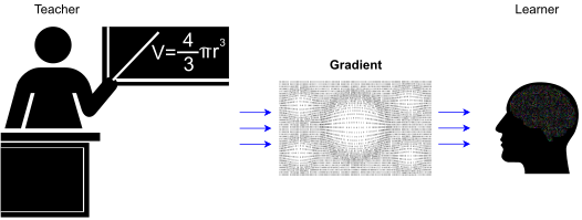
Solution: use gradient-based techniques
13.4 Gradient-Based Learning
Gradient Descent
Gradient Descent Algorithm
Objective: minimize a objective function (cost function) J(\boldsymbol{\theta})=J(\theta_{1},\theta_{2},...,\theta_{D}) \begin{equation} \hat{\boldsymbol{\theta}}=\arg\min_{\boldsymbol{\theta}}J(\boldsymbol{\theta}) \end{equation}
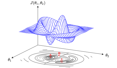
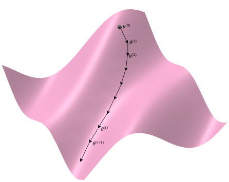
Gradient descent method: an iterative procedure where, at each iteration i we modify the parameters \boldsymbol{\theta}
Init \boldsymbol{\theta}^{(0)}
Do until satisfied
update \boldsymbol{\theta} to reduce J(\boldsymbol{\theta}) \begin{equation} \boldsymbol{\theta}^{(t+1)}\leftarrow\boldsymbol{\theta}^{(t)}-{\color{green}\eta}\nabla_{\boldsymbol{\theta}}J \end{equation} where {\color{green}\eta} is learning rate (0<{\color{green}\eta}<1) and \begin{equation} \nabla_{\boldsymbol{\theta}}J=\left[\frac{\partial J}{\partial\theta_{1}},\frac{\partial J}{\partial\theta_{2}},\cdots,\frac{\partial J}{\partial\theta_{D}}\right]^{\intercal} \end{equation}
Gradient descent variants
There are three variants of gradient descent. Depending on the amount of data, we make a trade-off between the accuracy of the parameter update and the time it takes to perform an update.
Batch gradient descent
Stochastic gradient descent
Mini-batch gradient descent
Batch gradient descent
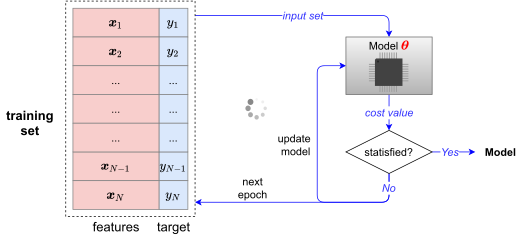
- Batch gradient descent (vanilla gradient descent) computes the gradient of the cost function w.r.t. to the parameters \boldsymbol{\theta} for the entire training dataset \mathcal{D}=\{(\boldsymbol{x}_{1},y_{1}),(\boldsymbol{x}_{2},y_{2})...(\boldsymbol{x}_{N},y_{N})\} \begin{equation} \boldsymbol{\theta}_{t+1}=\boldsymbol{\theta}_{t}-{\color{green}\eta}\cdot\nabla_{\boldsymbol{\theta}}J(\boldsymbol{\theta}_{t}\mid\mathcal{D}) \end{equation}
Cons
We need to calculate the gradients for the whole dataset to perform just one update
It can be very slow and is intractable for datasets that do not fit in memory.
It also does not allow us to update our model online, i.e. with new examples on-the-fly.
Stochastic gradient descent
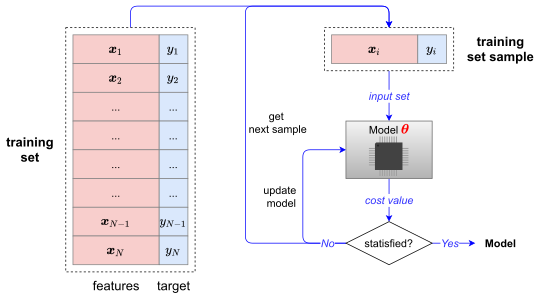
Stochastic gradient descent (SGD) in contrast performs a parameter update for each training example \boldsymbol{x}_{i} and label y_{i} of the training dataset \mathcal{D}=\{(\boldsymbol{x}_{1},y_{1}),(\boldsymbol{x}_{2},y_{2})...(\boldsymbol{x}_{N},y_{N})\} \begin{equation} \boldsymbol{\theta}_{t+1}=\boldsymbol{\theta}_{t}-{\color{green}\eta}\cdot\nabla_{\boldsymbol{\theta}}J(\boldsymbol{\theta}_{t}\mid\boldsymbol{x}_{i},y_{i}) \end{equation}
Note that we should shuffle the training data at every epoch
Cons
- SGD performs frequent updates with a high variance that cause the objective function to fluctuate heavily

Mini-batch gradient descent
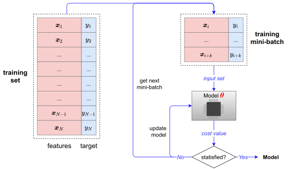
- Mini-batch gradient descent finally takes the best of both worlds and performs an update for every mini-batch of k training examples of the training dataset \mathcal{D}=\{(\boldsymbol{x}_{1},y_{1}),(\boldsymbol{x}_{2},y_{2})...(\boldsymbol{x}_{N},y_{N})\} \begin{equation} \boldsymbol{\theta}_{t+1}=\boldsymbol{\theta}_{t}-{\color{green}\eta}\cdot\nabla_{\boldsymbol{\theta}}J(\boldsymbol{\theta}_{t}\mid\boldsymbol{x}_{i:i+k},y_{i:i+k}) \end{equation}
Pros
It reduces the variance of the parameter updates, which can lead to more stable convergence
It can make use of highly optimized matrix optimizations common to state-of-the-art deep learning libraries that make computing the gradient w.r.t. a mini-batch very efficient.
Gradient Ascent
Gradient Ascent
- Objective: maximize a objective function (cost function) J(\boldsymbol{\theta})=J(\theta_{1},\theta_{2},...,\theta_{D}) \begin{equation} \hat{\boldsymbol{\theta}}=\arg\max_{\boldsymbol{\theta}}J(\boldsymbol{\theta}) \end{equation}
Min-max optimization
Min-max
- Objective: Given a objective function (cost function) J(x,y)
\begin{equation} \hat{x},\hat{y}=\arg\min_{x}\max_{y}J(x,y) \end{equation}
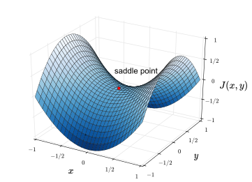
- GAN optimization (original version), does not always converge
13.5 Advanced Gradient-Based Learning
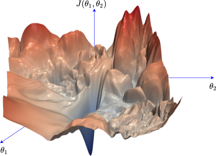
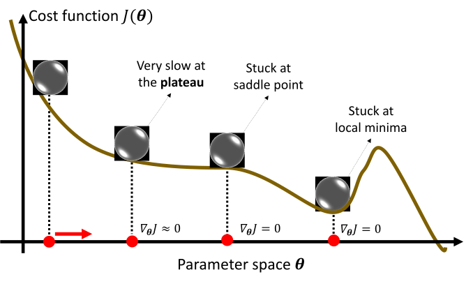
Gradient descent: Local minima
Gradient descent never guarantee global minima
- Different initial point \boldsymbol{\theta}^{(0)} \to reach different minima, so different results
More issues of gradient descent
- It also has issues at plateau and saddle point
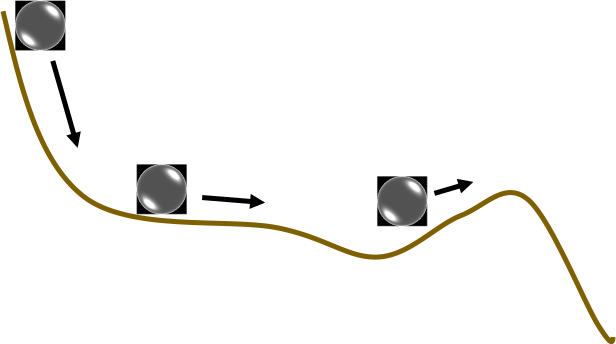
Momentum in physical world
- How about put this phenomenon in gradient descent?
Momentum
- Still not guarantee reaching global minima, but give some hope ...
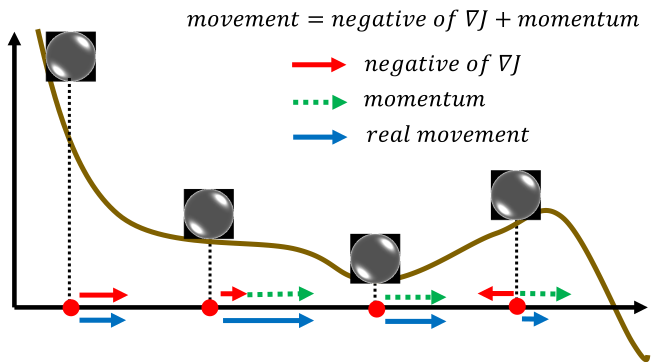
Momentum
Momentum is a method that helps accelerate SGD in the relevant direction and dampens oscillations
It does this by adding a fraction {\color{green}\gamma} of the update vector of the past time step to the current update vector
\begin{align} \begin{split}\boldsymbol{v}_{0} & =\boldsymbol{0}\\ \boldsymbol{v}_{t} & ={\color{green}\gamma}\boldsymbol{v}_{t-1}+{\color{green}\eta}\nabla_{\boldsymbol{\theta}}J(\boldsymbol{\theta}_{t-1})\\ \boldsymbol{\theta}_{t} & =\boldsymbol{\theta}_{t-1}-\boldsymbol{v}_{t} \end{split} \end{align}
- The momentum term {\color{green}\gamma} is usually set to 0.9 or a similar value.
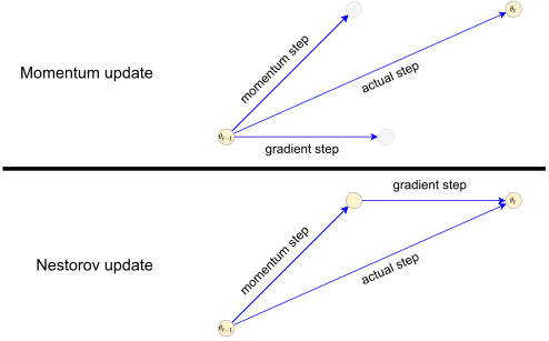
Nesterov accelerated gradient (NAG)
A ball that rolls down a hill, blindly following the slope, is highly unsatisfactory. We would like to have a smarter ball, a ball that has a notion of where it is going so that it knows to slow down before the hill slopes up again.
We can now effectively look ahead by calculating the gradient not w.r.t. to our current parameters \boldsymbol{\theta} but w.r.t. the approximate future position of our parameters:
\begin{align} \begin{split}\boldsymbol{v}_{0} & =\boldsymbol{0}\\ \boldsymbol{v}_{t} & ={\color{green}\gamma}\boldsymbol{v}_{t-1}+{\color{green}\eta}\nabla_{\boldsymbol{\theta}}J(\boldsymbol{\theta}_{t-1}-{\color{green}\gamma}\boldsymbol{v}_{t-1})\\ \boldsymbol{\theta}_{t} & =\boldsymbol{\theta}_{t-1}-\boldsymbol{v}_{t} \end{split} \end{align}
Adagrad
- Previously, we performed an update for all parameters \boldsymbol{\theta} at once as every parameter \theta_{i} used the same learning rate {\color{green}\eta}. As Adagrad (Duchi, 2011) uses a different learning rate for every parameter \theta_{i} at every time step t \begin{equation} \theta_{t+1,i}=\theta_{t,i}-\eta_{t,i}\cdot g_{t,i} \end{equation} where \begin{equation} g_{t,i}=\frac{\partial J}{\partial\theta_{t,i}} \end{equation} and \eta_{t,i}=\frac{{\color{green}\eta}}{\sqrt{\sum_{k=0}^{t}g_{k,i}^{2}}}
Pros
- One of Adagrad’s main benefits is that it eliminates the need to manually tune the learning rate {\color{green}\eta}. Most implementations use a default value of 0.01 and leave it at that.
Cons
- Since every added term is positive, the accumulated sum keeps growing during training. This in turn causes the learning rate to shrink and eventually become infinitesimally small, at which point the algorithm is no longer able to acquire additional knowledge.
Other Learning Methods rather than Adagrad
Adadelta (Zeiler, 2012) is an extension of Adagrad that seeks to reduce its aggressive, monotonically decreasing learning rate. Instead of accumulating all past squared gradients, Adadelta restricts the window of accumulated past gradients to some fixed size w.
RMSprop is an adaptive learning rate method proposed by Geoff Hinton.
Adadelta
Adam
AdaMax
Nadam
13.6 Back-propagation Learning
Computational Graph
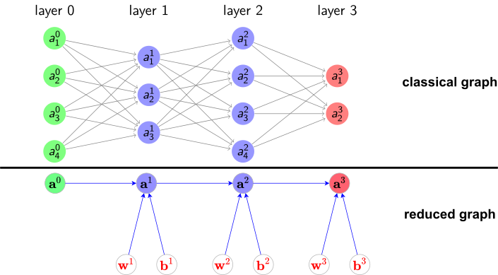
The classical graph of neural network is cumbersome at first, and it does take some work to master
We use the another reperesentaion, reduced graph (computational graph)
The back-propagation algorithm
Proposed by Bryson and Ho, 1969 \to most popular among over a hundred different learning algorithms available.
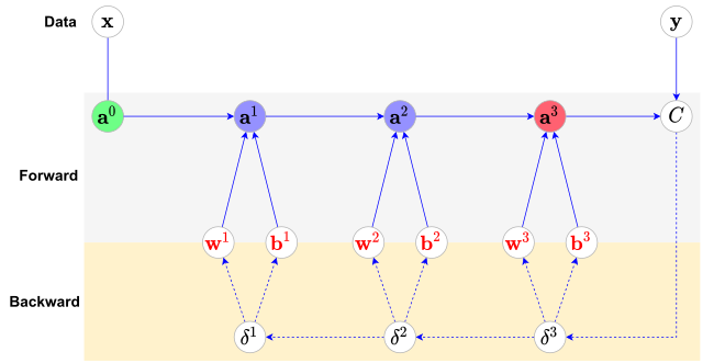
The algorithm provide us with a way of computing the gradient of the cost function C({\color{red}\boldsymbol{w}},\boldsymbol{{\color{red}b}}).
Input (\boldsymbol{x},\boldsymbol{y}): Set the corresponding activation \boldsymbol{a}^{0} for the input layer.
Feedforward:
Init \boldsymbol{a}^{0}=\boldsymbol{x}
For each l=1,2,\ldots,L compute \begin{equation} \boldsymbol{z}^{l}={\color{red}\boldsymbol{w}^{l}}\boldsymbol{a}^{l-1}+{\color{red}\boldsymbol{b}^{l}}\qquad\text{and}\qquad\boldsymbol{a}^{l}=\sigma(\boldsymbol{z}^{l}) \end{equation} where \sigma is an activation function
Compute the cost value C
Backpropagate:
Compute the error vector \boldsymbol{\delta}^{L} \begin{equation} \boldsymbol{\delta}^{L}=\sigma'(\boldsymbol{z}^{L})\odot\nabla C \end{equation}
For each l=L-1,L-2,\ldots,1, compute the error vector \boldsymbol{\delta}^{l} \begin{equation} \boldsymbol{\delta}^{l}=(({\color{red}\boldsymbol{w}}^{l+1})^{\intercal}\boldsymbol{\delta}^{l+1})\odot\sigma'(\boldsymbol{z}^{l}) \end{equation}
Compute the partial gradient of the cost function with respect to parameters \begin{equation} \frac{\partial C}{\partial{\color{red}w_{jk}^{l}}}=a_{k}^{l-1}\delta_{j}^{l}\qquad\text{and}\qquad\frac{\partial C}{\partial{\color{red}b_{j}^{l}}}=\delta_{j}^{l} \end{equation}