14  DEEP NEURAL NETWORKS

14.1 History

Ups & Downs of Neural Networks

NNs and AI have experienced several hype cycles, followed by disappointment, criticism, and funding cuts:

• 1950s - 70s: Golden years of AI (funded by DARPA): solve algebra, play chess & checkers, reasoning, semantic nets “within ten years a digital computer will be the world’s chess champion”

• 1969: shown that XOR problem cannot be solved by Perceptron (led to the invention of multi-layer networks later on)

• Mid 1970s: Chain reaction that begins with pessimism in the AI community, followed by pessimism in the press, followed by a severe cutback in funding, followed by the “end” of serious research (“AI winter”)

• 1980s: Governments (starting in Japan) and industry provide AI with billions of dollars. Boom of “expert systems”.

• 1986: Backpropagation had been invented in the 1970s, but only 1986 it became popular through a famous paper by David Rumelhart, Geoffrey Hinton, and Ronald Williams. It showed that also complex functions became solvable through NNs by using multiple layers.

• Late 1980s: Investors - despite actual progress in research - became disillusioned and withdrew funding again.

Why no Deep Learning in the 1980s?

Neural Networks could not become “deep” yet - because:

• Computers were slow. So the neural networks were tiny and could not achieve (the expected) high performance on real problems.

• Datasets were small. There were no large datasets that had enough information to constrain the numerous parameters of (hypothetical) large neural networks.

• Nobody knew how to train deep nets. Today, object recognition networks have > 25 successive layers of convolutions. In the past, everyone was very sure that such deep nets cannot be trained. Therefore, networks were shallow and did not achieve good results.

Ups & Downs of Neural Networks

• 1991: Hornik proved 1 hidden layer network can model any continuous function (universal approximation theorem)

• 1991-1992: Vanishing Gradient, problem in multi-layer networks where training in front layers is slow due to backpropagation diminishing the gradient updates through the layers. Identified by Hochreiter & Schmidhuber who also proposed solutions.

• 1990s - mid 2000s: Due to lack of computational power, interest in NNs decreased again and other Machine Learning models, such as Bayesian models, Decision Trees and Support Vector Machines became popular.

Resurrection of Deep Learning

• 2000s: Hinton, Bengio and LeCun (“The fathers of the age of deep learning”) join forces in a project. They overcome some problems that caused deep networks not to learn anything at all

• 2006: Breakthrough with Layer-wise pre-training by unsupervised learning (using RBMs)

• 2010s - present: Important new contributions:

  • Simpler initialization (without pre-training)

  • Dropout

  • Simplier activations: Rectifier Units (ReLUs)

  • Batch Normalization

  \to not a re-invention of NNs but paved the way for very deep NNs

14.2 Architecture

Deep Learning vs. Classical Machine Learning

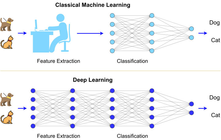
Deep neural network (DNN)

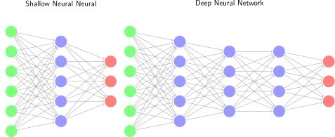
• Deep neural networks (DNNs) are basically ANNs with multiple hidden layers between the input and output layers.

Activation functions

Activation functions

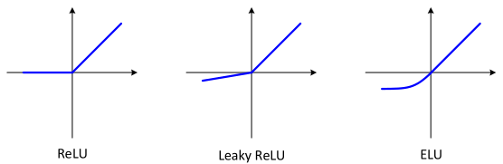
• ReLU function \begin{equation} a=\text{ReLU}(x)=\max(0,x)=\begin{cases} x & x\geq0\\ 0 & x<0 \end{cases} \end{equation}

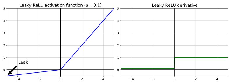
• Leaky ReLU function \begin{equation} a=\text{LeakyReLU}(x)=\max(\alpha x,x)=\begin{cases} x & x\geq0\\ \alpha x & x<0 \end{cases} \end{equation}

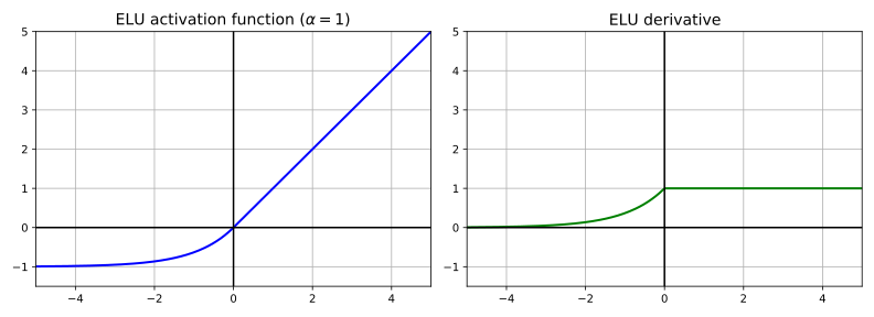
• ELU function \begin{equation} a=\text{ELU}(x)=\begin{cases} x & x\geq0\\ \alpha(\exp(x)-1) & x<0 \end{cases} \end{equation}

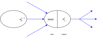
Maxout Gate

• The maxout unit takes a group of input activations and ouput the maximum value

\begin{equation} f(\boldsymbol{x})=f(x_{1},x_{2},...,x_{k})=\max_{i}(x_{i}) \end{equation}

Why Deep?

Why Deep?

Experiment

• Deep networks are empirically better in solving many real-world problems

• Deep networks is providing breakthrough results in speech recognition and image classification

  Network	Error	Layers
  AlexNet	16.0%	8
  ZFNet	11.2%	8
  VGGNet	7.3%	19
  GoogLeNet	6.7%	22
  MS ResNet	3.6%	152!

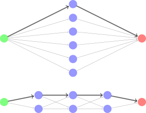
Analogy

Logic circuits	Neural network
Logic circuits consists of gates	Neural network consists of neurons
A two layers of logic gates can represent any Boolean function.	A hidden layer network can represent any continuous function.
Using multiple layers of logic gates to build some functions are much simpler	Using multiple layers of neurons to represent some functions are much simpler
\to less gates needed	\to less parameters

Another reason

Learning with DNNs

• Feature hierarchies (feature engineering) are learnt such that features from higher levels formed by the composition of lower level features.

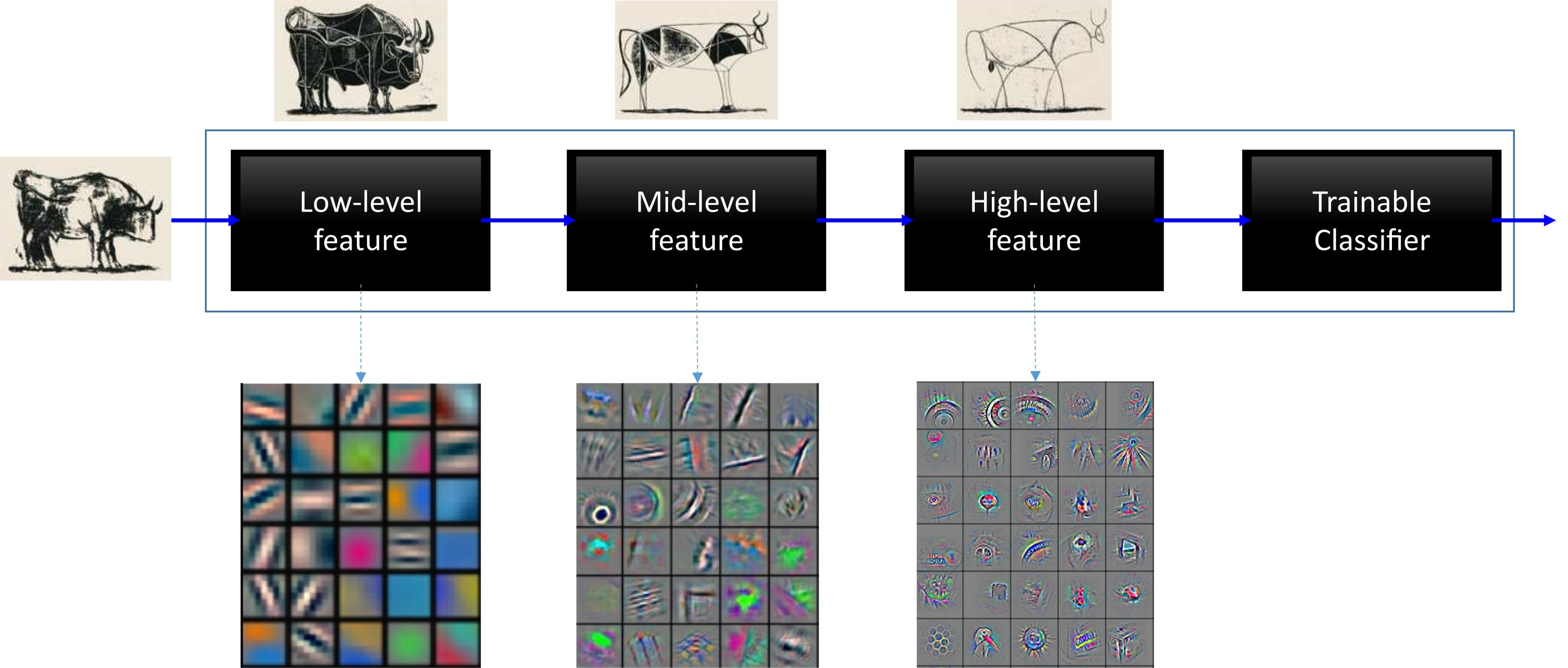
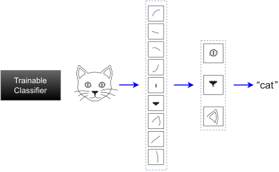
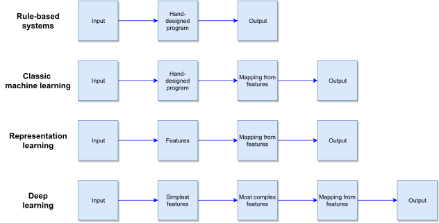
Learning Multiple Levels of Abstraction

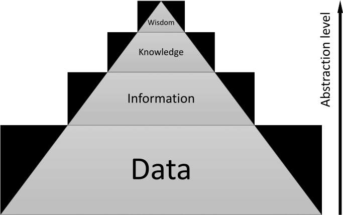
• The big payoff of deep learning is to allow learning higher levels of abstraction

• Higher-level abstractions disentangle the factors of variaton, which allows much easier generalization and transfer

Types of Deep neural networks

• Convolutional neural network (CNN)

• Recurrent Neural Networks (RNN)

• Autoencoders

• Generative Adversarial Nets (GAN)

• Region Based CNN (R-CNN)

• YOLO

• RNN ConvNet

• BERT Models

• GPT Models

• Transformer Models

14.3 Design

Deep Learning Framework

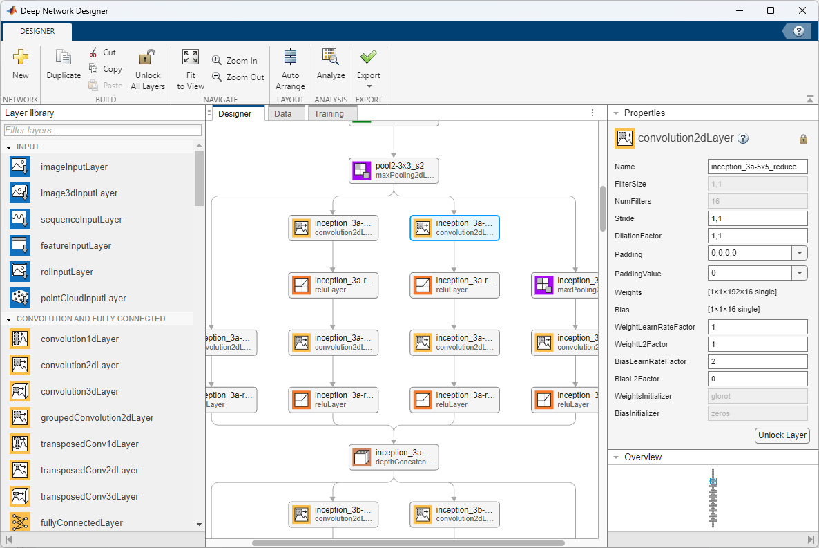
Design by GUI

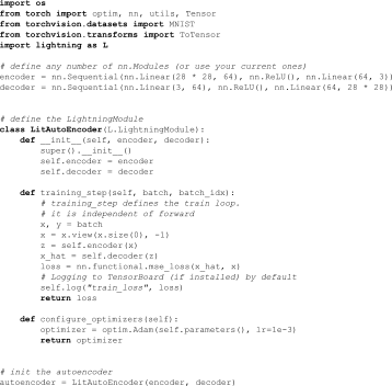
Design by Code

14.4 Visualization

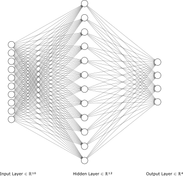
MLP Style

Lenet Style

• 2.5 D style

• Lenet

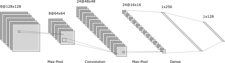
Alex Style

• 3D style

• Alexnet

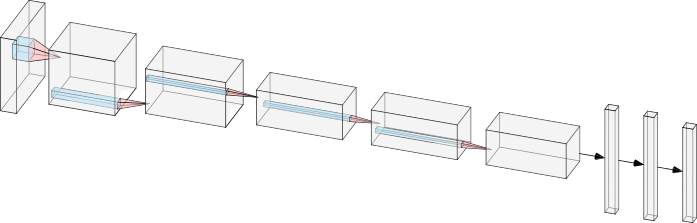
Simple Style

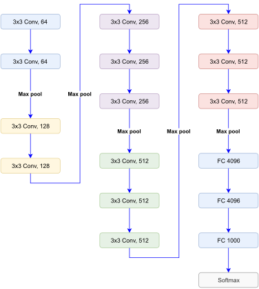
• 2D style

• VGG16 has 16 layers, not counting the maxpool layers and the softmax at the end

14.5 Learning Problem

Why are deep neural networks hard to train?

• There’s an intrinsic instability associated to learning by gradient descent in many-layer (deep) neural networks

• This instability tends to result in either the early or the later layers getting stuck during training

  • The vanishing gradient problem and

  • The opposite of this problem is called the exploding gradient problem

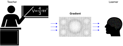
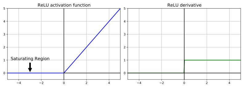
Vanishing gradient problem

The vanishing gradient problem

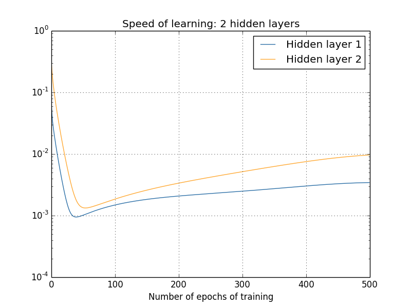
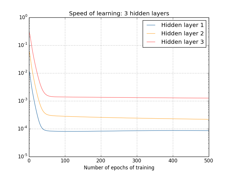
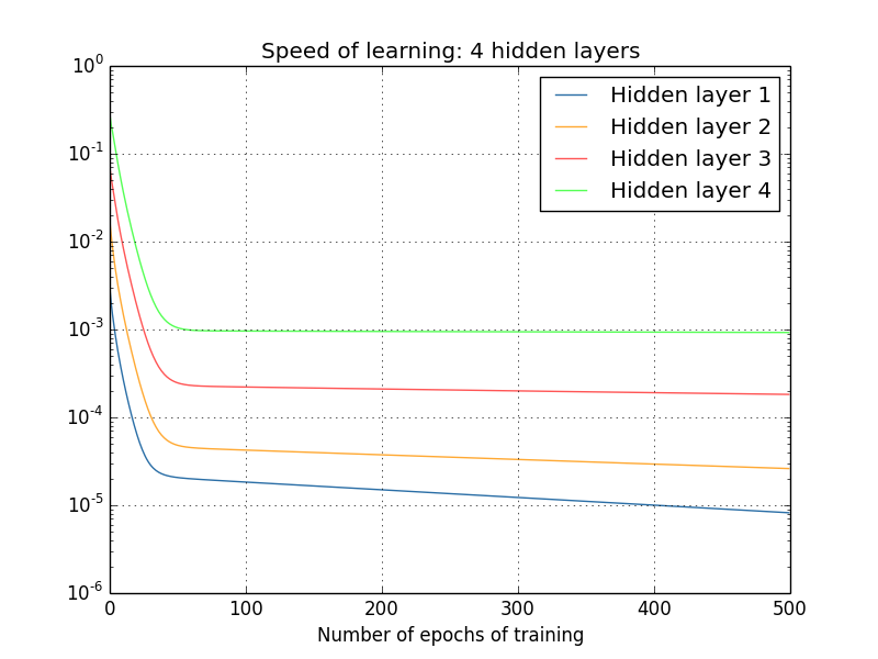
What’s causing the vanishing gradient problem?

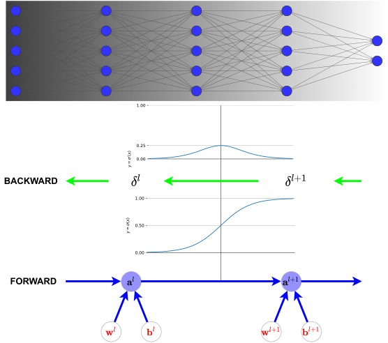
Nonsaturating Activation Functions

ReLU

Rectified linear units (ReLU) allow for faster and effective training of DNNs on large and complex datasets.

• Biological plausibility

  • One-sided, compared to the anti-symmetry of \tanh

• Sparse activation

  • E.g., in a randomly initialized network, only about 50% of hidden units are activated (having a non-zero output)

• Better gradient propagation

  • Fewer vanishing gradient problems compared to sidgmoid activation functions that saturate in both directions

• Efficient computation: Only comparison

• Scale-invariant \forall x,\max(0,ax)=a\max(0,x)

How does a ReLU work?

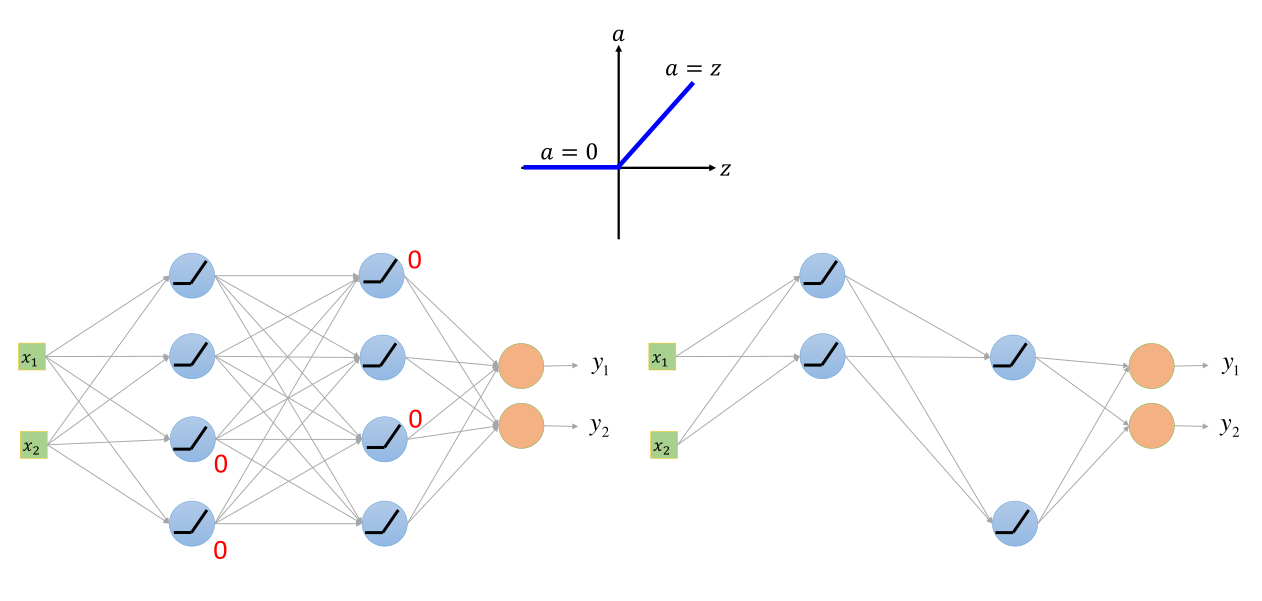
ReLU: Potential issues

• Non-differentiable at zero

  • However, it is differentiable anywhere else, including points arbitrarily close to (but not equal to) zero.

• Non-zero centered

• Unbounded

• Dying ReLU problem

Dropout

Dropout

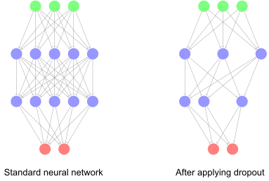
• Dropout is a technique for regularization. Unlike L_{1} and L_{2} regularization, dropout doesn’t rely on modifying the cost function. Instead, in dropout we modify the network structure itself.

Training Procedure

For each mini-batch

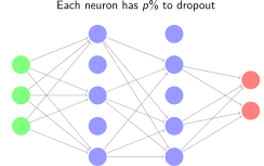
• Start by randomly (and temporarily) deleting p\% the hidden neurons in the network, while leaving the input and output neurons untouched

• We forward-propagate the input through the modified network, and then back-propagate the result to update the appropriate weights and biases

Testing Procedure

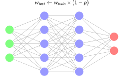
Using original neural network, no dropout

• If the dropout rate at training is p\%, all the weights times (1-p)\%; e.g., assume that the dropout rate is p=40\%, if a weight w_{train}=1 by training, set w_{test}=0.6 for testing

Why it works

There two ways of understanding why this works

• This makes the network unable to relay on a single feature

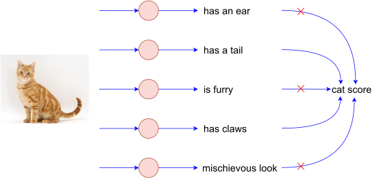
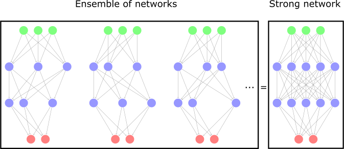
• It can also be seen as training a large ensemble of models that share parameters

Batch Normalization

Batch Normalization

• Batch normalization reparametrizes the model to make artificial neural networks faster and more stable

• Key idea: normalize, shift and rescale data

• Learning

  Input:	Values of x over a training set mini-batch, each of size m: \mathcal{B}=\{x^{(1..m)}\}
  	Parameters to be learned: {\color{red}\gamma}, {\color{red}\beta}
  Output:	\{y^{(i)}=\textrm{BN}_{{\color{red}\gamma},{\color{red}\beta}}(x^{(i)})\}
  	{\color{red}\mu}_{\mathcal{B}}\leftarrow{\displaystyle \frac{1}{m}{\displaystyle \sum_{i=1}^{m}x^{(i)}}} (mini-batch mean)
  	{\color{red}\sigma}_{\mathcal{B}}^{2}\leftarrow{\displaystyle \frac{1}{m}{\displaystyle \sum_{i=1}^{m}(x^{(i)}-{\color{red}\mu}_{\mathcal{B}})^{2}}} (mini-batch variance)
  	\hat{x}^{(i)}\leftarrow{\displaystyle \frac{x^{(i)}-{\color{red}\mu}_{\mathcal{B}}}{\sqrt{{\color{red}\sigma}_{\mathcal{B}}^{2}+\epsilon}}} (normalize)
  	y^{(i)}\leftarrow{\color{red}\gamma}\hat{x}^{(i)}+{\color{red}\beta} (scale and shift)

• Inference

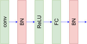
  Input:	x
  Output:	y
  	\text{E}(x)\gets\text{E}_{\mathcal{B}}[{\color{red}\mu}_{\mathcal{B}}]
  	\text{Var}(x)\gets\dfrac{m}{m-1}\text{E}_{\mathcal{B}}[{\color{red}\sigma}_{\mathcal{B}}^{2}]
  	y=\dfrac{{\color{red}\gamma}}{\sqrt{\text{Var}(x)+\epsilon}}x+\left({\color{red}\beta}-\dfrac{{\color{red}\gamma}\text{E}(x)}{\sqrt{\text{Var}(x)+\epsilon}}\right)

• Common configuration: insert BN layers right after Conv or FC layers, before ReLU layers

14.6 Workflow

Metrics

Confusion matrix

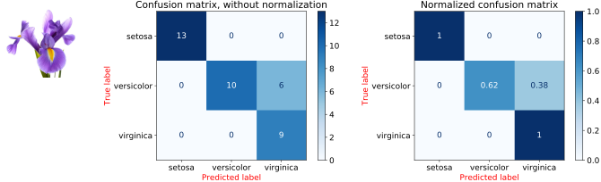
• Each column of the matrix represents the instances in a predicted class while each row represents the instances in an actual class

Two-class confusion matrix

Consider two-class problem with two classes \oplus and \ominus

• Number of true positives TP

• Number of true negatives TN

• Number of false positives FP

• Number of false negatives FN

• The number of actual positives P=TP+FN

• The number of actual negatives N=TN+FP

  	Predicted \oplus	Predicted \ominus
  Actual \oplus	TP	FN
  Actual \ominus	FP	TN

Example

• Let’s assume we are building a binary classification to classify cat/non-cat(\oplus/\ominus) images. And let’s assume our test set has 1100 images (1000 non-cat images, and 100 cat images), with the below confusion matrix.

  	Predicted cat	Predicted non-cat
  Actual cat	90	10
  Actual non-cat	60	940

Classification related metrics

Accuracy (acc) is the number of correct predictions divided by the total number of predictions. \begin{equation} acc=\frac{TP+TN}{P+N} \end{equation} Error rate (err) is defined as \begin{equation} err=1-acc \end{equation}

acc=\frac{90+940}{1000+100}=93.6\%\text{ and }err=1-acc=6.4\%

• Accuracy is considered as a weighted average

• There are many cases in which classification accuracy is not a good indicator of your model performance. One of these scenarios is when your class distribution is imbalanced

Precision (pre) is defined as \begin{equation} pre=\frac{TP}{TP+FP} \end{equation}

pre_{\text{cat}}=\frac{90}{90+60}=60\%\text{ and }pre_{\text{non-cat}}=\frac{940}{940+10}=98.9\%

Sensitivity (recall, hit rate, or true positive rate tpr) is defined as the fraction of samples from class \oplus which are correctly predicted by the model \begin{equation} tpr=\frac{TP}{P}. \end{equation} Specificity (selectivity or true negative rate tnr) is defined as the fraction of samples from class \ominus which are correctly predicted by the model \begin{equation} tnr=\frac{TN}{N} \end{equation}

tpr_{\text{cat}}=\frac{90}{100}=90\%\text{ and }tpr_{\text{non-cat}}=\frac{940}{1000}=94\%

• Depending on application, you may want to give higher priority to sensitivity or precision.

• But there are many applications in which both sensitivity and precision are important.

F1-score (F_{1}) is defined as the harmonic mean of precision and sensitivity \begin{equation} F_{1}=\frac{2\times precision\times sensitivity}{precision+sensitivity} \end{equation}

F_{1\text{cat}}=\frac{2\times0.6\times0.9}{0.6+0.9}=72\%

Fall-out or false positive rate (fpr) is defined as \begin{equation} fpr=\frac{FP}{N} \end{equation}

ROC Curve

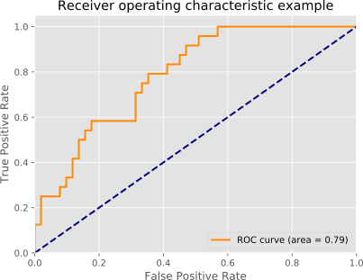
• The receiver operating characteristic (ROC) curve is plot which shows the performance of a binary classifier as function of its cut-off threshold.

• It essentially shows the true positive rate (tpr) against the false positive rate (fpr) for various threshold values.

• The area under the curve (AUC) is an aggregated measure of performance.

Regression related metrics

“Mean squared error” (MSE) is the average squared error between the predicted and actual values. MSE=\frac{1}{n}\sum_{i=1}^{n}(y_{i}-\hat{y}_{i})^{2}

Workflow

Workflow

Important Question: How well a system will do on new, unseen data?

The workflow includes

1. Selecting features and collecting data.

2. Choosing a performance metric.

3. Choosing a classifier and optimization algorithm.

4. Evaluating the performance of the model.

5. Tuning the algorithm.

Prepare Data

Data

• Collecting data

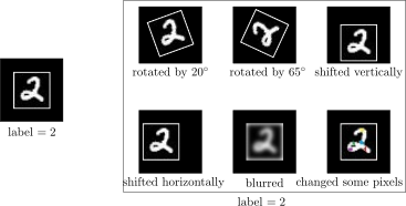
• Artificially augmenting the data

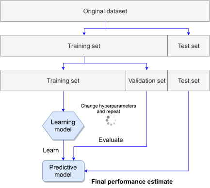
• Splitting the data into three independent sets: training, validation, and test

  • We train on the training set and evaluate our model on the validation set. Once our model is ready for prime time, we test it one final time on the test set.

  • An essential rule of the training and testing process is that we never learn from the test data.

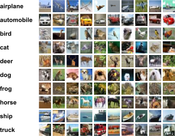
Data augmentation

• Geometric: flipping, rotation, shearing, multiple crops

• Photometric: color transformations

• Other: add noise, compression artifacts, lens distortions, etc.

Data preprocessing

• Zero centering

  • Subtract mean image – all input images need to have the same resolution

  • Subtract per-channel means – images don’t need to have the same resolution

• Optional: rescaling – divide each value by (per-pixel or per-channel) standard deviation

• Be sure to apply the same transformation at training and test time!

  • Save training set statistics and apply to test data

Choose Metric

Performance metric

Identify Needs

• High accuracy or low accuracy?

  • Surgery robot: high accuracy

  • Celebrity look-a-like app: low accuracy

Choose Metrics

• Accuracy? (% of examples correct)

• Coverage? (% of examples processed)

• Precision? (% of detections that are right)

• Recall? (% of objects detected)

• Amount of error? (For regression problems)

Choose Model

Model

Deep or Not?

• Lots of noise, little structure \to not deep

  • Logistic regression, SVM, boosted tree are all good

• Little noise, complex structure \to deep

What Architecture?

• No structure \to fully connected

• Spatial structure \to convolutional

• Sequential structure \to recurrent

• Mixed structure \to our design

Train Model

Hold-out validation

• If we have much data

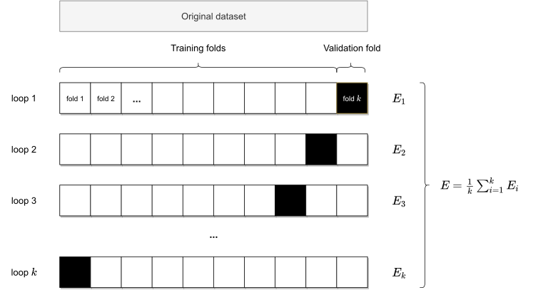
K-fold validation

• If we don’t have much data

Sanity test

• Make sure that the model can overfit very small portion of the training data.

• Take \approx 20 samples, turn off regularization and make sure that model can get a loss of 0 (accuracy 100%).

  • If model can’t overfit there is a problem: or there is something broken or we have to scale up your network.

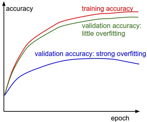
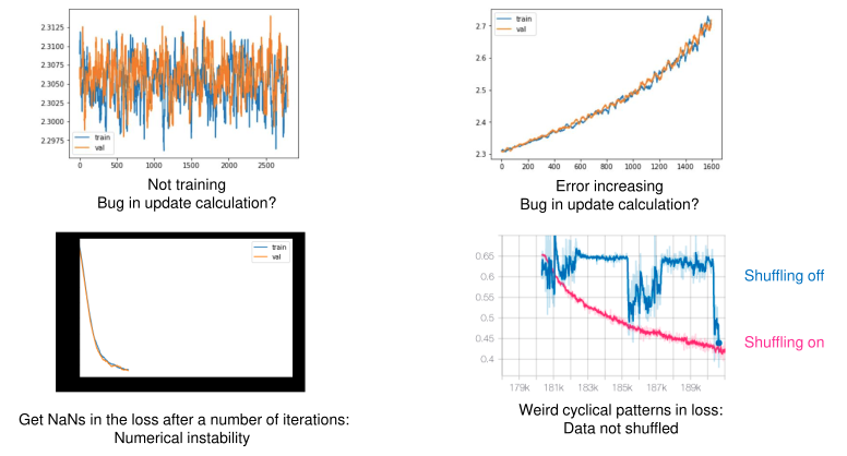
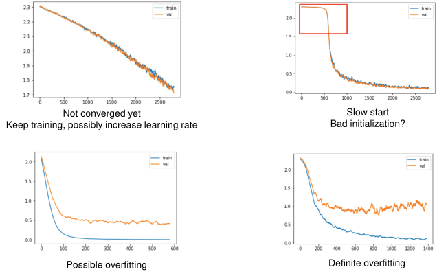
Monitor learning curves

The gap between the training and validation accuracy indicates the amount of overfitting

• Gap between train-validation is too big: overfitting, increase regularization

• Gap between train-validation too small: increase model capacity

When to stop training?

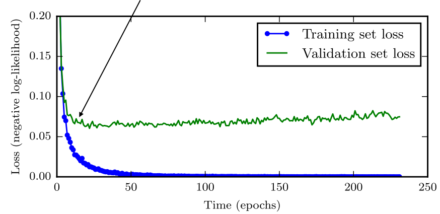
• Monitor validation error to decide when to stop

  • “Patience” hyperparameter: number of epochs without improvement before stopping

  • Early stopping: terminate while validation set performance is better (a kind of regularization)

  

Other techniques

• Track the ratio of weight updates and weight magnitudes. \begin{equation} r=\frac{weight\_updates}{weight\_magnitudes}~ \end{equation}

  • If this is too high to decrease learning rate

  • If it is too low to increase learning rate

• If dropout is not working for model, we should probably be using a bigger network.

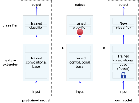
Using a pretrained model

A pretrained network is a saved network that was previously trained on a large dataset

• A common and highly effective approach to deep learning on small image datasets is to use a pretrained network.

• There are two ways to use a pretrained network: feature extraction and fine-tuning.

Essential Skills to ML scientists/engineers

• Design a model

• Run + Debug the model

• Revise the model

14.7 References