19 REINFORCEMENT LEARNING
Agent and Environment
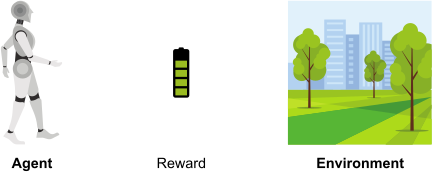
Agent: takes actions.
Environment: the world in which the agent exists and operates.
Reward: feedback that measures the success or failure of the agent’s action.
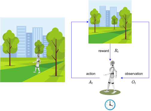
At each step t the agent:
Executes action A_{t}
Receives observation O_{t}
Receives scalar reward R_{t}
The environment:
Receives action A_{t}
Emits observation O_{t+1}
Emits scalar reward R_{t+1}
t increments at env. step
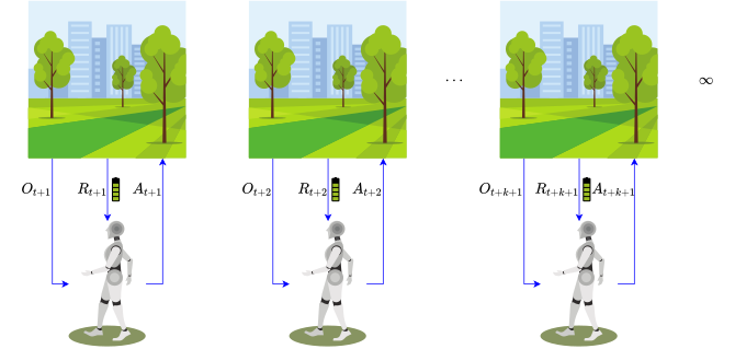
Total reward obtained from time t \begin{equation} G_{t}=\sum_{k=0}^{\infty}R_{t+k+1}=R_{t+1}+R_{t+2}+\cdots \end{equation}
Discounted total reward with discount factor \gamma \begin{equation} G_{t}=\sum_{k=0}^{\infty}\gamma^{k}R_{t+k+1}=R_{t+1}+\gamma R_{t+2}+\cdots \end{equation}
Reinforcement Learning
Reinforcement learning (RL) is concerned with how intelligent agents ought to take actions in an environment in order to maximize the notion of cumulative reward
Consider learning to choose actions, e.g.,
Robot learning to dock on battery charger
Learning to choose actions to optimize factory output
Learning to play Backgammon
Note several problem characteristics:
Delayed reward
Opportunity for active exploration
Possibility that state only partially observable
Possible need to learn multiple tasks with same sensors/effectors
Characteristics of Reinforcement Learning
What makes reinforcement learning different from other machine learning paradigms?
There is no supervisor, only a reward signal
Feedback is delayed, not instantaneous
Time really matters (sequential, non i.i.d data)
Agent’s actions affect the subsequent data it receives
19.1 The Reinforcement Learning Problem
19.2 Problems
Cart-Pole Problem
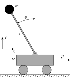
Objective: Balance a pole on top of a movable cart
State: angle, angular speed, position, horizontal velocity
Action: horizontal force applied on the cart
Reward: 1 at each time step if the pole is upright
Robot Locomotion
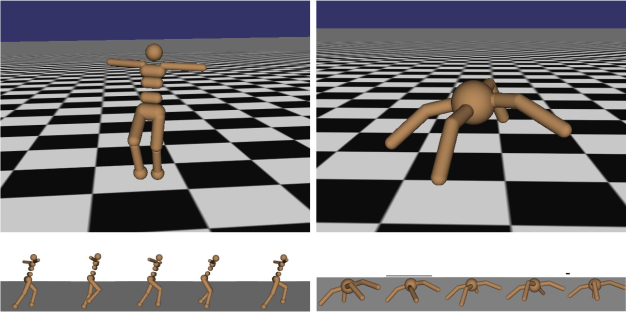
Objective: Make the robot move forward
State: Angle, position, velocity of all joints
Action: Torques applied on joints
Reward: 1 at each time step upright + forward movement
Atari Games
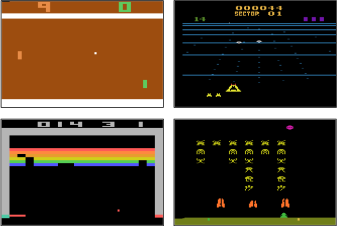
Objective: Complete the game with the highest score
State: Raw pixel inputs of the game screen
Action: Game controls e.g. Left, Right, Up, Down
Reward: Score increase/decrease at each time step
Go
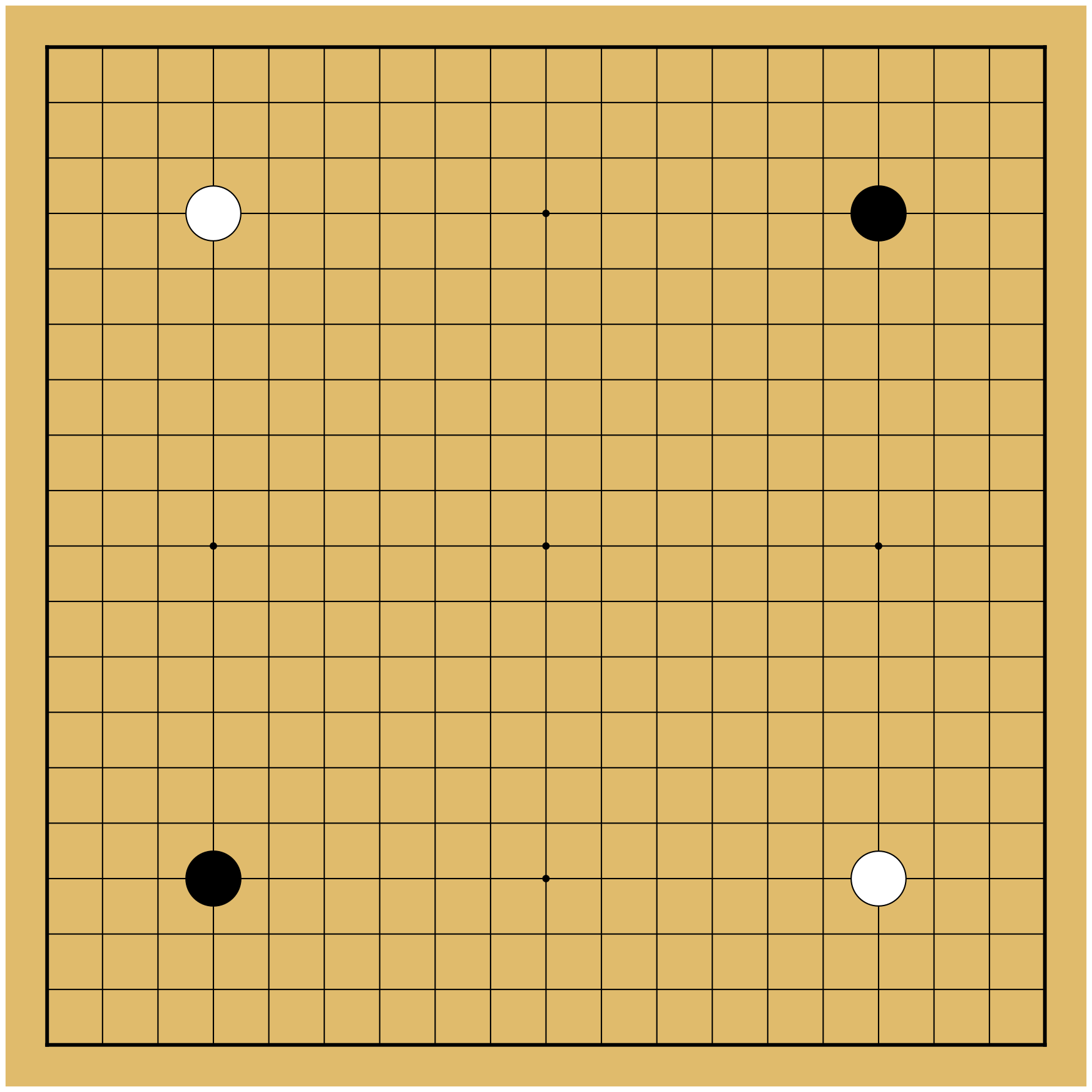
Objective: Win the game!
State: Position of all pieces
Action: Where to put the next piece down
Reward: On last turn: 1 if you won, 0 if you lost
19.3 State
History and State
The history is the sequence of observations, actions, rewards, i.e. all observable variables up to time t \begin{equation} H_{t}=O_{1},R_{1},A_{1},...,A_{t-1},O_{t},R_{t} \end{equation}
What happens next depends on the history:
The agent selects actions
The environment selects observations/rewards
State is the information used to determine what happens next. Formally, state is a function of the history \begin{equation} S_{t}=f(H_{t}) \end{equation}
Environment State
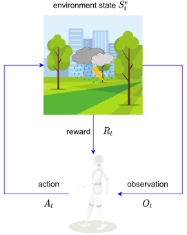
The environment state S_{t}^{e} is the environment’s private representation
i.e. whatever data the environment uses to pick the next observation/reward
The environment state is not usually visible to the agent
Even if S_{t}^{e} is visible, it may contain irrelevant information
Agent State
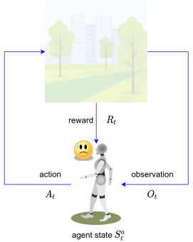
The agent state S_{t}^{a} is the agent’s internal representation
i.e. whatever information the agent uses to pick the next action
i.e. it is the information used by reinforcement learning algorithms
It can be any function of history: \begin{equation} S_{t}^{a}=f(H_{t}) \end{equation}
Information State
An information state (a.k.a. Markov state) contains all useful information from the history.
A state S_{t} is Markov if and only if \begin{equation} P[S_{t+1}\mid S_{t}]=P[S_{t+1}\mid S_{1},...,S_{t}] \end{equation}
- “The future is independent of the past given the present”
\begin{equation} H_{1:t}\to S_{t}\to H_{t+1:\infty} \end{equation}
- Once the state is known, the history may be thrown away; i.e., the state is a sufficient statistic of the future
Markov Assumption
The environment state S_{t}^{e} is Markov
The history H_{t} is Markov
Fully Observable Environments
Full observability: agent directly observes environment state \begin{equation} O_{t}=S_{t}^{a}=S_{t}^{e} \end{equation}
- Formally, this is a Markov decision process (MDP)
Partially Observable Environments
Partial observability: agent indirectly observes environment; now agent state is different from environment state. Agent must construct its own state representation S_{t}^{a} , e.g.
Complete history: S_{t}^{a}=H_{t}
Beliefs of environment state: S_{t}^{a}=(P[S_{t}^{e}=s^{1}],...,P[S_{t}^{e}=s^{n}])
Recurrent neural network: S_{t}^{a}=\sigma(S_{t-1}^{a}W_{s}+O_{t}W_{o})
A robot with camera vision isn’t told its absolute location
A trading agent only observes current prices
A poker playing agent only observes public cards
Formally this is a partially observable Markov decision process (POMDP)
19.4 Inside An RL Agent
Major Components of an RL Agent
An RL agent may include one or more of these components:
Agent state
Policy: agent’s behaviour function
Value function: how good is each state and/or action
Model: agent’s representation of the environment
Policy
A policy is the agent’s behaviour. It is a map from state to action
Deterministic policy: \begin{equation} a=\pi(s) \end{equation}
Stochastic policy: \begin{equation} \pi(a\mid s)=P[A_{t}=a\mid S_{t}=s] \end{equation}
Value Function
Value function is a prediction of future reward
Used to evaluate the goodness/badness of states
And therefore to select between actions, e.g.
\begin{equation} v_{\pi}(s)=\mathbb{E}_{\pi}[R_{t+1}+\gamma R_{t+2}+\gamma^{2}R_{t+3}+...\mid S_{t}=s] \end{equation}
Model
A model predicts what the environment will do next
- \mathcal{P} predicts the next state
\begin{equation} \mathcal{P}_{ss'}^{a}=P[S_{t+1}=s'\mid S_{t}=s,A_{t}=a] \end{equation}
- \mathcal{R} predicts the next (immediate) reward \begin{equation} \mathcal{R}_{s}^{a}=\mathbb{E}[R_{t+1}\mid S_{t}=s,A_{t}=a] \end{equation}
Maze Example
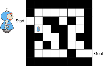
Rewards: -1 per time-step
Actions: N, E, S, W
States: Agent’s location
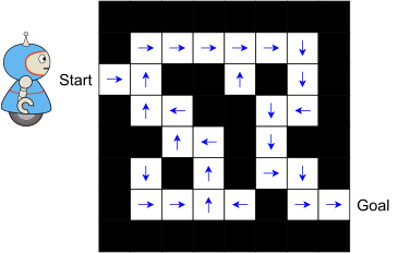
Maze Example: Policy
- Arrows represent policy \pi(s) for each state s
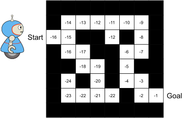
Maze Example: Value Function
- Numbers represent value v^{\pi}(s) of each state s
Maze Example: Model
Agent may have an internal model of the environment
Dynamics: how actions change the state
Rewards: how much reward from each state
The model may be imperfect
Grid layout represents transition model P_{ss'}^{a}
Numbers represent immediate reward R_{s}^{a} from each state s (same for all a)
Categorizing RL agents
|
|
19.5 Problems within Reinforcement Learning
Learning and Planning
Two fundamental problems in sequential decision making
Reinforcement Learning:
The environment is initially unknown
The agent interacts with the environment
The agent improves its policy
Planning:
A model of the environment is known
The agent performs computations with its model (without any external interaction)
The agent improves its policy
Atari Example: Reinforcement Learning
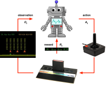
Rules of the game are unknown
Learn directly from interactive game-play
Pick actions on joystick, see pixels and scores
Atari Example: Planning
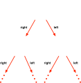
Rules of the game are known
Can query emulator
- perfect model inside agent’s brain
If I take action a from state s:
what would the next state be?
what would the score be?
Plan ahead to find optimal policy
- e.g. tree search
Exploration and Exploitation
Reinforcement learning is like trial-and-error learning
The agent should discover a good policy
from its experiences of the environment
without losing too much reward along the way
Exploration finds more information about the environment
Exploitation exploits known information to maximise reward
It is usually important to explore as well as exploit
Exploration and exploitation (cont.)
| Exploitation | Exploration | |
|---|---|---|
| go with the best strategy found so far | take a new action with unknown consequences | |
| Pros | Maximize reward as reflected in the current utility estimates | Get a more accurate model of the environment |
| Avoid bad stuff | Discover higher-reward states than the ones found so far | |
| Cons | Might also prevent you from discovering the true optimal strategy | When you’re exploring, you’re not maximizing your utility |
| Something bad might happen |
Examples

| Exploitation | Exploration | |
|---|---|---|
| Restaurant Selection | Go to your favourite restaurant | Try a new restaurant |
| Online Banner Advertisements | Show the most successful advert | Show a different advert |
| Oil Drilling | Drill at the best known location | Drill at a new location |
| Game Playing | Play the move you believe is best | Play an experimental move |
Prediction and Control
Prediction: evaluate the future
- Given a policy
Control: optimise the future
- Find the best policy
19.6 Agent’s Learning Task
Value Functions
The state-value function at state s, is the expected cumulative reward from following the policy \pi from state s \begin{equation} v^{\pi}(s)=\mathbb{E}\left[G_{t}\mid S_{t}=s\right] \end{equation}
The action-value Q function at state s and action a, is the expected cumulative reward from taking action a in state s and then following the policy \pi \begin{equation} q^{\pi}(s,a)=\mathbb{E}\left[G_{t}\mid S_{t}=s,A_{t}=a\right] \end{equation}
Optimal Value Functions
The optimal state-value function v^{*}(s) is the maximum value function over all policies \begin{equation} v^{*}(s)=\max_{\pi}v^{\pi}(s) \end{equation}
The optimal action-value function q^{*}(s,a) is the maximum action-value function over all policies \begin{equation} q^{*}(s,a)=\max_{\pi}q^{\pi}(s,a) \end{equation}
Estimating Value Functions
Estimating v^{\pi} or q^{\pi} is called policy evaluation or, simply, prediction
Estimating v^{*} or q^{*} is sometimes called control, because these can be used for policy optimization
Optimal Policy
A partial ordering over policies \begin{equation} \pi\geq\pi'\text{ if }v^{\pi}(s)\geq v^{\pi'}(s),\forall s \end{equation}
For any Markov Decision Process
There exists an optimal policy \pi^{\ast} that is better than or equal to all other policies, \pi^{\ast}\geq\pi,\forall\pi
All optimal policies achieve the optimal value function, v^{\pi^{\ast}}(s)=v^{\ast}(s)
All optimal policies achieve the optimal action-value function, q^{\pi^{\ast}}(s,a)=q^{\ast}(s,a)
Agent’s Learning Task
- Agent’s Goal: Find the optimal policy \pi^{\ast} that maximize the expected sum of rewards . \begin{equation} \pi^{\ast}=\arg\max_{\pi}\mathbb{E}\left[G_{t}\right] \end{equation}
Optimal Q-function
q^{\ast} encodes the optimal policy, an optimal policy can be found by maximising over q^{\ast}(s,a) \begin{equation} \pi^{\ast}(a\mid s)=\begin{cases} 1 & \text{if }a=\arg\max_{a\in\mathcal{A}}q^{\ast}(s,a)\\ 0 & \text{otherwise} \end{cases} \end{equation} \begin{equation} \pi^{\ast}(s)=\arg\max_{a}q^{\ast}(s,a) \end{equation}
If we know q^{\ast}(s,a), we immediately have the optimal policy
19.7 Bellman Equation
Bellman equations
Two Bellman equations for policy \pi \begin{align} v^{\pi}(s) & =\mathbb{E}[R_{t+1}+\gamma v^{\pi}(S_{t+1})\mid S_{t}=s]\\ q^{\pi}(s,a) & =\mathbb{E}[R_{t+1}+\gamma q^{\pi}(S_{t+1},A_{t+1})\mid S_{t}=s,A_{t}=a]\nonumber \end{align}
Two Bellman optimality equations
\begin{align} v^{\ast}(s) & =\max_{a}\mathbb{E}[R_{t+1}+\gamma v^{\ast}(S_{t+1})\mid S_{t}=s,A_{t}=a]\\ q^{\ast}(s,a) & =\mathbb{E}[R_{t+1}+\gamma\max_{a'}q^{\ast}(S_{t+1},a')\mid S_{t}=s,A_{t}=a]\nonumber \end{align}
Bellman equations (cont.)
- There are equivalences between state and action values \begin{align} v^{\pi}(s) & =\sum_{a}\pi(a\mid s)q^{\pi}(s,a)\\ v^{\ast}(s) & =\max_{a}q^{\ast}(s,a) \end{align}
Solving the Bellman Optimality Equation
Bellman Optimality Equation is non-linear and there is no closed form solution (in general)
Many iterative solution methods
Using models/dynamic programming
Value iteration
Policy iteration
Using samples
Monte Carlo
Q-learning
Sarsa
19.8 Dynamic Programming
What is Dynamic Programming?
Dynamic Programming is a method for solving complex problems by breaking them down into subproblems
Solve the subproblems
Combine solutions to subproblem
- All such methods consist of two important parts: policy evaluation and policy improvement
Requirements for Dynamic Programming
Dynamic Programming is a very general solution method for problems which have two properties:
Optimal substructure
Principle of optimality applies
Optimal solution can be decomposed into subproblems
Overlapping subproblems
Subproblems recur many times
Solutions can be cached and reused
19.9 Q-Learning
Q-Learning for Deterministic Worlds
For each (s,a) initialize table entry Q(s,a)\leftarrow0
Observe current state s
Do forever:
Select an action a and execute it
Receive immediate reward r and observe the new state s'
Update the table entry for Q(s,a) as follows \begin{align} Q(s,a) & \leftarrow r+\gamma\max_{a'}Q(s',a')\\ s & \leftarrow s'\nonumber \end{align}
Q-Learning Theorem
Notice if rewards non-negative, then (\forall s,a,n)\ 0\leq Q_{n}(s,a)\leq Q_{n+1}(s,a)\leq Q^{\ast}(s,a)
Q converges to Q^{\ast}.
Proof. Proof. Define a full interval to be an interval during which each (s,a) is visited. During each full interval the largest error in Q table is reduced by factor of \gamma
Let Q_{n} be table after n updates, and \Delta_{n} be the maximum error in Q_{n}; that is \Delta_{n}=\max_{s,a}|Q_{n}(s,a)-Q^{\ast}(s,a)|
For any table entry Q_{n}(s,a) updated on iteration n+1, the error in the revised estimate Q_{n+1}(s,a) is
\begin{align*} |Q_{n+1}(s,a)-Q^{\ast}(s,a)| & = & |(r+\gamma\max_{a'}Q_{n}(s',a'))-(r+\gamma\max_{a'}Q^{\ast}(s',a'))|\\ & = & \gamma|\max_{a'}Q_{n}(s',a')-\max_{a'}Q^{\ast}(s',a')|\\ & \leq & \gamma\max_{a'}|Q_{n}(s',a')-Q^{\ast}(s',a')|\\ & \leq & \gamma\max_{s'',a'}|Q_{n}(s'',a')-Q^{\ast}(s'',a')|\\ |Q_{n+1}(s,a)-Q^{\ast}(s,a)| & \leq & \gamma\Delta_{n} \end{align*} ◻
Q-Learning for Nondeterministic Worlds
For each (s,a) initialize table entry Q(s,a)\leftarrow0
Iterate over t=1,2,\dotsc
\qquadUpdate the table entry for Q(s,a) as follows \begin{align} Q^{new}(s_{t},a_{t})\leftarrow & Q(s_{t},a_{t})+\nonumber \\ & \underset{\text{learning rate}}{\underbrace{\alpha}}\overset{\text{temporal difference}}{\overbrace{[\underset{\text{new value}}{\underbrace{r_{t}+\gamma\max_{a}Q(s_{t+1},a)}}-\underset{\text{old value}}{\underbrace{Q(s_{t},a_{t})}}]}} \end{align}
- Q converges to Q^{\ast} [Watkins and Dayan, 1992]