3 LINEAR MODEL
Notation
| symbol | meaning |
|---|---|
| a,b,c,N\dots | scalar number |
| \boldsymbol{w},\boldsymbol{v},\boldsymbol{x},\boldsymbol{y}\dots | column vector |
| \boldsymbol{X},\boldsymbol{Y}\dots | matrix |
| \mathbb{R} | set of real numbers |
| \mathbb{Z} | set of integer numbers |
| \mathbb{N} | set of natural numbers |
| \mathbb{R}^{D} | set of vectors |
| \mathcal{X},\mathcal{Y},\dots | set |
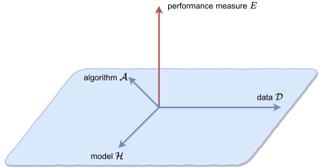
| \mathcal{A} | algorithm |
| operator | meaning |
|---|---|
| \boldsymbol{w}^{\intercal} | transpose |
| \boldsymbol{X}\boldsymbol{Y} | matrix multiplication |
| \boldsymbol{X}^{-1} | inverse |
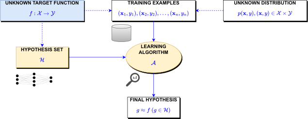
Learning diagram
3.1 Simple Linear Model
Problem 1
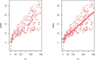
Consider the Advertising data set \mathcal{D}_{train} consists of the sales of that product in 200 different markets, along with advertising budgets for the product in each of those markets for the media TV. Find the relationship between TV (input) and sales (output)
Linear Regression Model
A linear regression is a model that assumes a linear relationship between inputs and the output.
Problem Statement
The requirement is to build a system that can take a vector \boldsymbol{x}\in\mathbb{R}^{D+1} as input and predict the value of a scalar y\in\mathbb{R} as its output
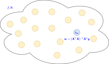
The hypothesis set \mathcal{H} y\approx\hat{y}=h_{{\color{red}\boldsymbol{w}}}(\mathbf{x})=\boldsymbol{{\color{red}w}}^{\intercal}\boldsymbol{x} where \hat{y} be the value that our model (function) predicts y and {\color{red}\boldsymbol{w}}\in\mathbb{R}^{D+1} is a vector of parameters of the model
Task T: to predict y from \boldsymbol{x} by outputting \hat{y}=h_{{\color{red}\boldsymbol{w}}}(\mathbf{x})=\boldsymbol{{\color{red}w}}^{\intercal}\boldsymbol{x}
The train set \mathcal{D}_{train} denoted as (\boldsymbol{X},\boldsymbol{y}) including N samples \{(\boldsymbol{x}_{1},y_{1}),(\boldsymbol{x}_{2},y_{2})\dots(\boldsymbol{x}_{N},y_{N})\}, construct the matrix \boldsymbol{X} and the vectors \boldsymbol{y} and \hat{\boldsymbol{y}} \underset{\text{input data matrix}}{\underbrace{\boldsymbol{X}=\left[\begin{array}{c} \boldsymbol{x}_{1}^{\intercal}\\ \boldsymbol{x}_{2}^{\intercal}\\ \vdots\\ \boldsymbol{x}_{N}^{\intercal} \end{array}\right]}},\quad\underset{\text{target vector}}{\underbrace{\boldsymbol{y}=\left[\begin{array}{c} y_{1}\\ y_{2}\\ \vdots\\ y_{N} \end{array}\right]}},\quad\underset{\text{output vector}}{\underbrace{\hat{\boldsymbol{y}}=\left[\begin{array}{c} \hat{y}_{1}\\ \hat{y}_{2}\\ \vdots\\ \hat{y}_{N} \end{array}\right]}}
- Performance measure P:
The mean squared error MSE_{train} of the model on the train set \mathcal{D}_{train} \begin{aligned} MSE_{train} & =\frac{1}{N}\left\Vert \hat{\boldsymbol{y}}-\boldsymbol{y}\right\Vert ^{2}=\frac{1}{N}\sum_{n=1}^{N}(\hat{y}_{n}-y_{n})^{2} \end{aligned}
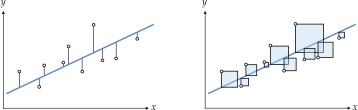
- The learning goal: find the vector of parameter \boldsymbol{{\color{red}w}} such that \boldsymbol{{\color{red}w}}=\arg\min_{\boldsymbol{{\color{red}w}}}(MSE_{train})
Solving Problem
Solution.
Compute the gradient of MSE_{train} \begin{aligned} \nabla_{\boldsymbol{{\color{red}w}}}(MSE_{train}) & = & \nabla_{\boldsymbol{{\color{red}w}}}(\boldsymbol{{\color{red}w}}^{\intercal}\boldsymbol{X}^{\intercal}\boldsymbol{X}\boldsymbol{{\color{red}w}}-\boldsymbol{{\color{red}w}}^{\intercal}\boldsymbol{X}^{\intercal}\boldsymbol{y}-\boldsymbol{y}^{\intercal}\boldsymbol{X}\boldsymbol{{\color{red}w}}+\boldsymbol{y}^{\intercal}\boldsymbol{y})\nonumber \\ & = & 2\boldsymbol{X}^{\intercal}\boldsymbol{X}\boldsymbol{{\color{red}w}}-2\boldsymbol{X}^{\intercal}\boldsymbol{y} \end{aligned}
If MSE_{train} reach the min value then \nabla_{\boldsymbol{{\color{red}w}}}(MSE_{train})=0 \begin{aligned} \nabla_{\boldsymbol{{\color{red}w}}}(MSE_{train}) & = & 0\nonumber \\ \boldsymbol{X}^{\intercal}\boldsymbol{X}\boldsymbol{{\color{red}w}}-\boldsymbol{X}^{\intercal}\boldsymbol{y} & = & 0\nonumber \\ \boldsymbol{X}^{\intercal}\boldsymbol{X}\boldsymbol{{\color{red}w}} & = & \boldsymbol{X}^{\intercal}\boldsymbol{y}\nonumber \\ \boldsymbol{{\color{red}w}} & = & (\boldsymbol{X}^{\intercal}\boldsymbol{X})^{-1}\boldsymbol{X}^{\intercal}\boldsymbol{y} \end{aligned}
◻
Programming Example
Use
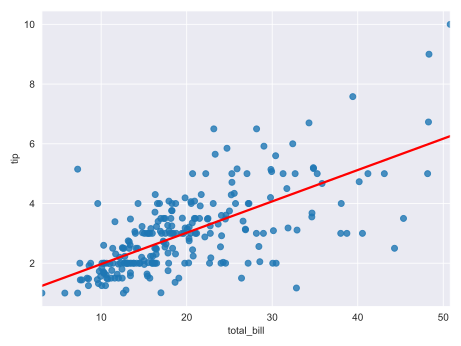
seabornto readtipsdataset and find the linear relationship betweentotal_billandtipimport numpy as np import seaborn as sns import matplotlib.pyplot as plt sns.set_style("darkgrid") tips = sns.load_dataset("tips") sns.regplot(x="total_bill", y="tip", data=tips, ci=None, line_kws={'color':'red'}) plt.show()
Word Example
Find the linear regression function y=f(x)={\color{red}w_{0}}+{\color{red}w_{1}}x given the following data set \mathcal{D}
input x target y 1 2 2 3 3 3 4 5 Find the linear regression function y=f(\boldsymbol{x})=f(x_{1},x_{2})={\color{red}w_{0}}+{\color{red}w_{1}}x_{1}+{\color{red}w_{2}}x_{2} given the following data set \mathcal{D}
input \boldsymbol{x} target y (1, 1) 1 (2, 3) 3 (3, 4) 4 (4, 3) 5
Discussion
D is a large number
Online learning
Limitations of the model (hypothesis set)
3.2 Weighted Linear Model
Weighted Linear Model
- In some cases the observations may be weighted; for example, they may not be equally reliable. In this case, we find the vector of parameters \boldsymbol{{\color{red}w}} to minimize the weighted sum of squares of errors \begin{aligned} E_{train} & =\sum_{n=1}^{N}a_{n}(\hat{y}_{n}-y_{n})^{2} \end{aligned}
Solving Problem
Construct the matrices \boldsymbol{X},\boldsymbol{A} and the vector \boldsymbol{y} \underset{\text{input data matrix}}{\underbrace{\boldsymbol{X}=\left[\begin{array}{c} \boldsymbol{x}_{1}^{\intercal}\\ \boldsymbol{x}_{2}^{\intercal}\\ \vdots\\ \boldsymbol{x}_{N}^{\intercal} \end{array}\right]}},\quad\underset{\text{weight matrix}}{\underbrace{\boldsymbol{A}=\left[\begin{array}{cccc} a_{1} & 0 & \cdots & 0\\ 0 & a_{2} & \cdots & 0\\ \vdots & \vdots & \ddots & \vdots\\ 0 & 0 & \cdots & a_{N} \end{array}\right]}},\quad\underset{\text{target vector}}{\underbrace{\boldsymbol{y}=\left[\begin{array}{c} y_{1}\\ y_{2}\\ \vdots\\ y_{N} \end{array}\right]}}
Calculate the vector of parameters \begin{array}{ccc} \boldsymbol{{\color{red}w}} & = & (\boldsymbol{X}^{\intercal}\boldsymbol{A}\boldsymbol{X})^{-1}\boldsymbol{X}^{\intercal}\boldsymbol{A}\boldsymbol{y}\end{array}
3.3 Linear Basis Function Model
Linear in What?
- Linearity in the weights h_{\boldsymbol{{\color{red}w}}}(\boldsymbol{x})={\color{red}w_{0}}+{\color{red}w}_{{\color{red}1}}x_{1}+...+{\color{red}w}_{{\color{red}D}}x_{D}
Linear Basis Function Models
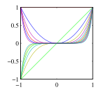
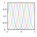
A linear basis function model is a linear combination of fixed nonlinear functions of the input variables h_{{\color{red}\boldsymbol{w}}}(\boldsymbol{x})={\color{red}w_{0}}\phi_{0}(\boldsymbol{x})+{\color{red}w_{1}}\phi_{1}(\boldsymbol{x})+...+{\color{red}w_{M}}\phi_{M}(\boldsymbol{x}) where \phi_{i}(\boldsymbol{x}) are basis functions
Some types of basis functions
Polynomial
\phi_{j}(x)=x^{j}
Gaussian
\phi_{j}(x;\mu_{j},s_{j})=\exp\left(-\frac{\left(x-\mu_{j}\right)^{2}}{s_{j}^{2}}\right)
Sigmoid
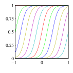
\phi_{j}(x;\mu_{j},s_{j})=\dfrac{1}{1+e^{-\frac{x-\mu_{j}}{s_{j}}}}
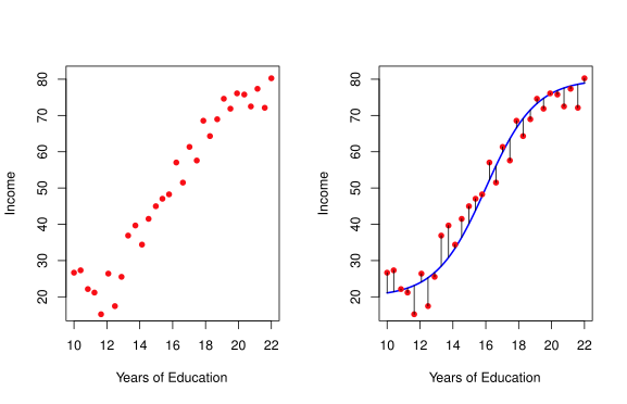
Problem 2
- Find the relationship between
Years of EducationandIncomebased on the given data
Problem Statement
The requirement is to build a system that can take a vector \boldsymbol{x}\in\mathbb{R}^{D} as input and predict the value of a scalar y\in\mathbb{R} as its output
The hypothesis set \mathcal{H} y\approx\hat{y}=h_{{\color{red}\boldsymbol{w}}}(\mathbf{x})=\boldsymbol{{\color{red}w}}^{\intercal}\boldsymbol{\phi}(\boldsymbol{x}) where \hat{y} be the value that our model (function) predicts y, {\color{red}\boldsymbol{w}}\in\mathbb{R}^{M+1} is a vector of parameters of the model and \boldsymbol{\phi} is a set of M+1 basis functions \boldsymbol{\phi}(\boldsymbol{x})=\left[\begin{array}{c} \phi_{0}(\boldsymbol{x})\\ \phi_{1}(\boldsymbol{x})\\ \vdots\\ \phi_{M}(\boldsymbol{x}) \end{array}\right]
Task T: to predict y from \boldsymbol{x} by outputting \hat{y}=h_{{\color{red}\boldsymbol{w}}}(\mathbf{x})=\boldsymbol{{\color{red}w}}^{\intercal}\boldsymbol{\phi}(\boldsymbol{x})
Performance measure P:
The mean squared error MSE_{train} of the model on the train set \mathcal{D}_{train} including N samples \{(\boldsymbol{x}_{1},y_{1}),(\boldsymbol{x}_{2},y_{2})\dots(\boldsymbol{x}_{N},y_{N})\}
The learning goal: find the vector of parameter \boldsymbol{{\color{red}w}} such that \boldsymbol{{\color{red}w}}=\arg\min_{\boldsymbol{{\color{red}w}}}(MSE_{train})
Solving Problem
Construct the matrix \boldsymbol{\Phi} and the vector \boldsymbol{y} \underset{\text{design matrix}}{\underbrace{\boldsymbol{\Phi}=\left[\begin{array}{c} \boldsymbol{\phi}(\boldsymbol{x}_{1})^{\intercal}\\ \boldsymbol{\phi}(\boldsymbol{x}_{2})^{\intercal}\\ \vdots\\ \boldsymbol{\phi}(\boldsymbol{x}_{N})^{\intercal} \end{array}\right]}},\quad\underset{\text{target vector}}{\underbrace{\boldsymbol{y}=\left[\begin{array}{c} y_{1}\\ y_{2}\\ \vdots\\ y_{N} \end{array}\right]}}
Calculate the vector of parameters \begin{array}{ccc} \boldsymbol{{\color{red}w}} & = & (\boldsymbol{\Phi}^{\intercal}\boldsymbol{\Phi})^{-1}\boldsymbol{\Phi}^{\intercal}\boldsymbol{y}\end{array}
Programming Example
import numpy as np
import seaborn as sns
import matplotlib.pyplot as plt

sns.set_style("darkgrid")
x = [1, 2, 3, 4, 5, 8, 10]
y = [1.1, 3.8, 8.5, 16, 24, 65, 99.2]
sns.regplot(x, y, order=2, ci=None, line_kws={'color':'red'})
plt.xlabel('x')
plt.ylabel('y')
plt.show()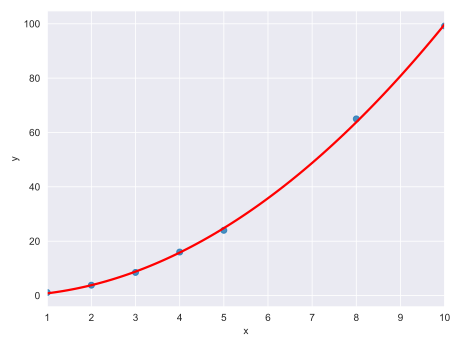
Word Example
Find a polynomial regression function y=f(x)={\color{red}w_{0}}+{\color{red}w_{1}}x+{\color{red}w_{2}}x^{2} given the data set \mathcal{D}
input x target y 1 2 2 3 3 3 4 5
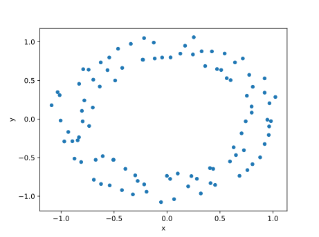
Puzzle
What basis functions?
3.4 Classification
A real data set
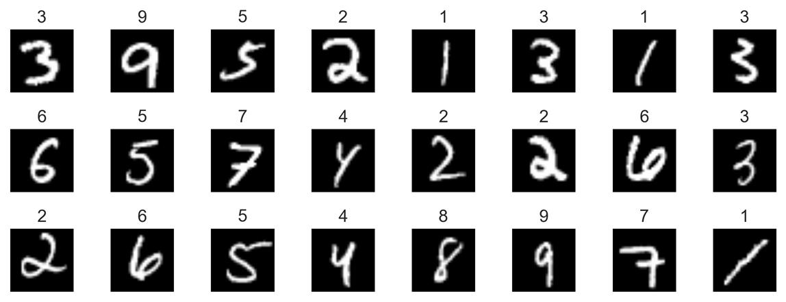
- Some 16-by-16 pixel grayscale image from the MNIST database
Input representation
Input representation or feature extraction
“raw” input
pixels \boldsymbol{x}^{\intercal}=\left(\begin{array}{cccc} x_{0} & x_{1} & \dots & x_{256}\end{array}\right) linear model \boldsymbol{{\color{red}w}}^{\intercal}=\left(\begin{array}{cccc} {\color{red}w_{0}} & {\color{red}w_{1}} & \dots & {\color{red}w}_{{\color{red}256}}\end{array}\right) Feature extraction: extract useful information
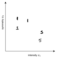
intensity and symmetry \boldsymbol{x}^{\intercal}=\left(\begin{array}{cc} x_{1} & x_{2}\end{array}\right) linear model \boldsymbol{{\color{red}w}}^{\intercal}=\left(\begin{array}{cc} {\color{red}w_{1}} & {\color{red}w}_{{\color{red}2}}\end{array}\right)
Illustration of Features
The Problem with Categorical Data
Some algorithms can work with categorical data directly.
- For example, a decision tree can be learned directly from categorical data with no data transform required
Many machine learning algorithms cannot operate on label data directly.
- They require all input variables and output variables to be numeric.
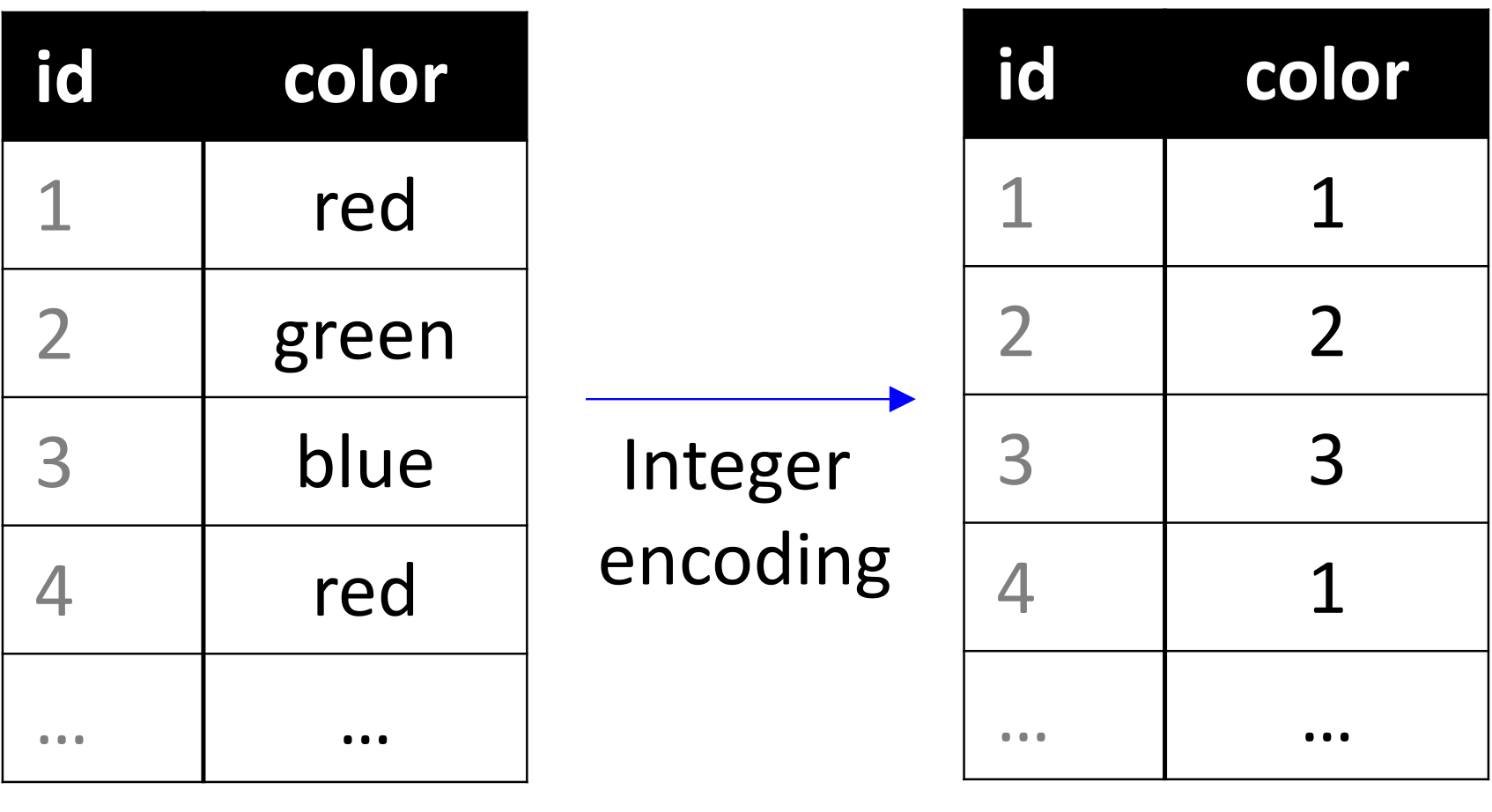
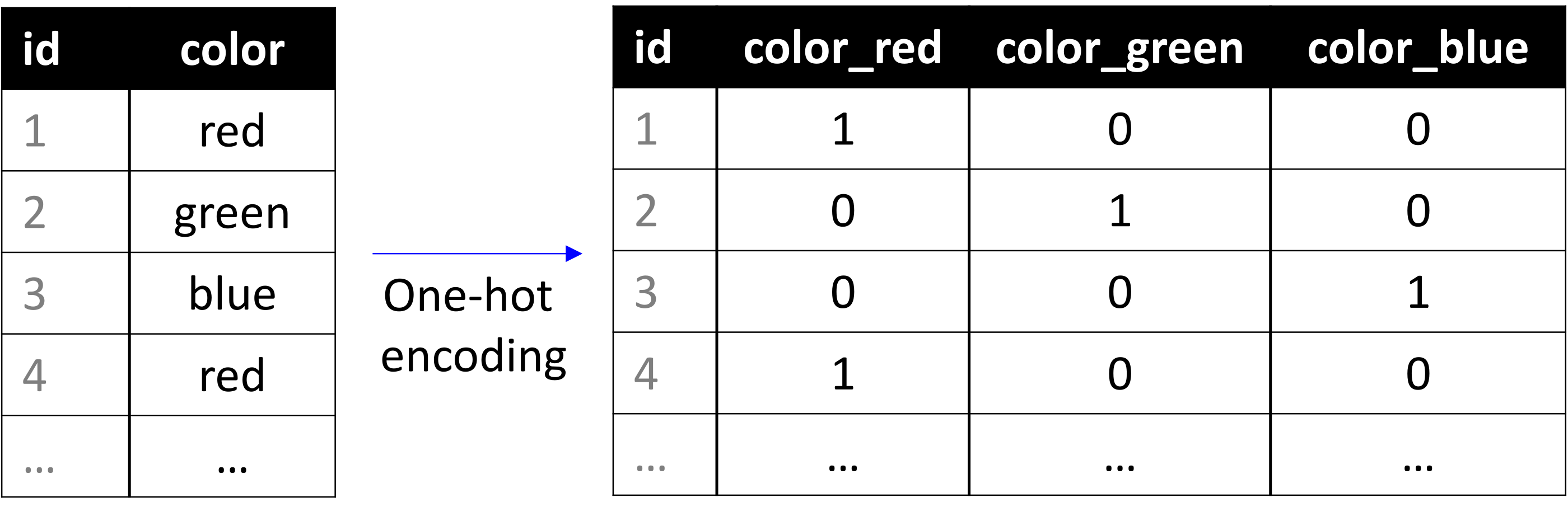
There are two common types of conversion: integer encoding and one-hot encoding
Integer Encoding
- For categorical variables where no such ordinal relationship exists, the integer encoding is not enough.
One-Hot Encoding
- One-hot encoding ensures that machine learning does not assume that higher numbers are more important.
Classifier Training
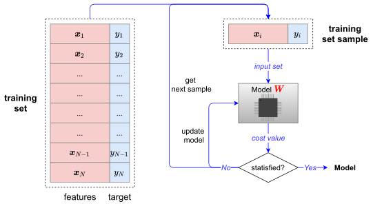
Select the learning model for classifier, e.g., Perceptron
Train the classifier/model using a training set \mathcal{D}=\{(\boldsymbol{x}_{1},y_{1}),...,(\boldsymbol{x}_{N},y_{N})\}
3.5 Logistic Regression
A Third Linear Model
s=\sum_{i=0}^{d}{\color{red}w_{i}}x_{i}
| linear classification | linear regression | logistic regression |
| h(\boldsymbol{x})=sign(s) | h(\boldsymbol{x})=s | h(\boldsymbol{x})=\sigma(s) |

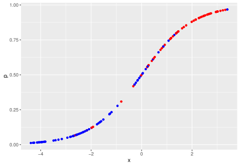
The logistic function
The formula \sigma(s)=\frac{1}{1+e^{-s}}
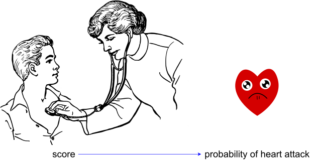
The logistic function converts a score to a probability
Properties
\sigma(-s)=1-\sigma(s)
\sigma^{\prime}(s)=\sigma(s)(1-\sigma(s))
Probability Interpretation
h(\boldsymbol{x})=\sigma(s) can be interpreted as a probability
For example, prediction of heart attacks
Input \boldsymbol{x}: cholesterol level, age, weight, etc.
The signal s=\boldsymbol{{\color{red}w}}^{T}\boldsymbol{x}: risk score
\sigma(s): probability of a heart attack
Problem Statement
The target function f is the probability distribution f:\mathbb{R}^{D}\to[0,1]
Hypothesis set h_{\boldsymbol{{\color{red}w}}}(\boldsymbol{x})=\sigma(\boldsymbol{{\color{red}w}}^{T}\boldsymbol{x}) and the conditional probability P(y\mid\boldsymbol{x},\boldsymbol{{\color{red}w}})=\left\{ \begin{array}{ccc} h_{\boldsymbol{{\color{red}w}}}(\boldsymbol{x}) & \text{for} & y=1\\ 1-h_{\boldsymbol{{\color{red}w}}}(\boldsymbol{x}) & \text{for} & y=0 \end{array}\right.
Error measure
We define error measurement based on likelihood
For each (\boldsymbol{x},y), y is generated by probability h_{\boldsymbol{{\color{red}w}}}(\boldsymbol{x}).
Plausible error measure based on likelihood of y given \boldsymbol{x} and {\color{red}\boldsymbol{w}} P(y\mid\boldsymbol{x},\boldsymbol{{\color{red}w}})=z^{y}(1-z)^{1-y} where z=h_{\boldsymbol{{\color{red}w}}}(\boldsymbol{x})=\sigma(\boldsymbol{{\color{red}w}}^{\intercal}\boldsymbol{x})
Likelihood of \mathcal{D}=\{(\boldsymbol{x}_{1},y_{1})...(\boldsymbol{x}_{N},y_{N})\} given {\color{red}\boldsymbol{w}} is \prod_{n=1}^{N}P(y_{n}\mid\boldsymbol{x}_{n},\boldsymbol{{\color{red}w}})
Learning goal: maximizing likelihood \begin{array}{ccc} & \text{Maximize} & \prod_{n=1}^{N}P(y_{n}\mid\boldsymbol{x}_{n},\boldsymbol{{\color{red}w}})\\ \Leftrightarrow & \text{Minimize} & -\log\prod_{n=1}^{N}P(y_{n}\mid\boldsymbol{x}_{n},\boldsymbol{{\color{red}w}})\\ \Leftrightarrow & \text{Minimize} & -\sum_{n=1}^{N}(y_{n}\log z_{n}+(1-y_{n})\log(1-z_{n})) \end{array}
Learning Algorithm (Gradient Descent)
Initialize the weights (parameters) at t=0 \boldsymbol{{\color{red}w}}_{0}
For t=1,2,3,... do
Compute the outputs z_{n} for each \boldsymbol{x}_{n} (n=1,...,N) \begin{equation} z_{n}=\sigma(\boldsymbol{{\color{red}w}}_{t}^{T}\boldsymbol{x}_{n}) \end{equation}
Compute the gradient \begin{equation} \nabla_{{\color{red}\boldsymbol{w}}}E=\frac{1}{N}\sum_{n=1}^{N}\boldsymbol{x}_{n}(z_{n}-y_{n}) \end{equation}
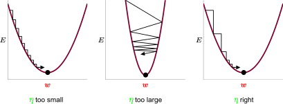
Update the weights \begin{equation} {\color{red}\boldsymbol{w}}_{t+1}=\boldsymbol{{\color{red}w}}_{t}-{\color{green}\eta}\nabla_{{\color{red}\boldsymbol{w}}}E \end{equation} where {\color{green}\eta} is a learning rate (hyper-parameter)
Iterate the next step until \boldsymbol{{\color{red}w}} is not changes
Return the final weights {\color{red}\boldsymbol{w}}
Learning Rate
How {\color{green}\eta} affects the algorithm?
Programming Example
import matplotlib.pyplot as plt
import seaborn as sns
sns.set(style="darkgrid")

# Load the example titanic dataset
df = sns.load_dataset("titanic")

# Make a custom palette with gendered colors
pal = dict(male="#6495ED", female="#F08080")

# Show the survival proability as a function of age and sex
g = sns.lmplot(x="age", y="survived", col="sex", hue="sex", data=df, palette=pal, y_jitter=.02, logistic=True, ci=None)
g.set(xlim=(0, 80), ylim=(-.05, 1.05))
plt.show()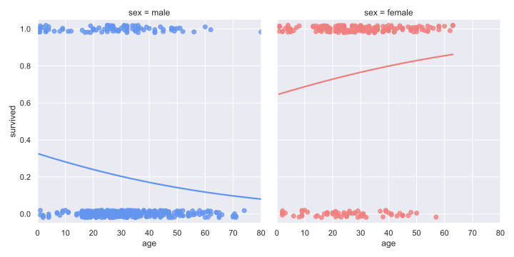
Evaluation
Consider two-class problem with two classes \oplus and \ominus
The performance of logistic regression model is based on a threshold th
\begin{aligned} y\text{ is } \oplus & \text{ if }P(y\mid\boldsymbol{x})\geq th\nonumber \\ y\text{ is } \ominus & \text{ if }P(y\mid\boldsymbol{x})<th \end{aligned}
High threshold: high specificity, low sensitivity
Low threshold: low specificity, high sensitivity
We should select the best threshold for the trade-off between the cost of false positives vs false negatives
ROC Curve
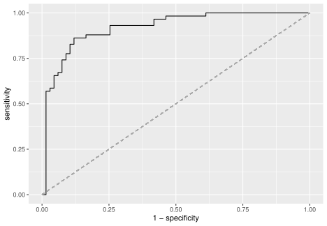
The receiver operating characteristic (ROC) curve is plot which shows the performance of a binary classifier as function of its cut-off threshold.
It essentially shows the true positive rate (sensitivity) against the false positive rate (1-specificity) for various threshold values.
The area under the curve (AUC) is an aggregated measure of performance.
Multi-class classification problems
Email foldering/tagging: Work (1), Friends (2), Family (3), Hobby (4)
Medical diagrams: Not ill, Cold, Flu
Weather: Sunny, Cloudy, Rain, Snow
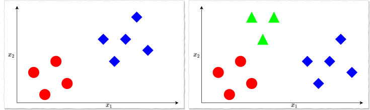
Visual of Binary vs Multi-class classification
Approaches
One-vs-one
Hierarchical
One-vs-all
One-vs-all
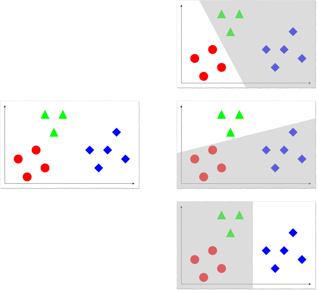
Class \circ (1): h^{(1)}(\boldsymbol{x})=P(y=1\mid\boldsymbol{x},\boldsymbol{{\color{red}w}}_{1})
Class \vartriangle (2): h^{(2)}(\boldsymbol{x})=P(y=2\mid\boldsymbol{x},\boldsymbol{{\color{red}w}}_{2})
Class \lozenge (3): h^{(3)}(\boldsymbol{x})=P(y=3\mid\boldsymbol{x},\boldsymbol{{\color{red}w}}_{3})
Learning
- Train a logistic regression classifier h^{(i)}(\boldsymbol{x}) for each class i to predict the probability that y=i.
Prediction
- On a new input \boldsymbol{x}, to make a prediction, pick the class i that maximizes \arg\max_{i}(h^{(i)}(\boldsymbol{x}))
Decision boundaries and decision regions
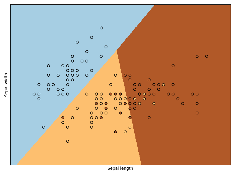
- Logistic regression for Iris dataset
3.6 Softmax Regression
Softmax Regression
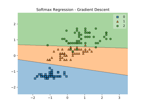
Softmax regression is a generalization of logistic regression that we can use for multi-class classification
- In Softmax regression, we replace the sigmoid function by the so-called softmax function \boldsymbol{\phi}(\cdot)=\{\phi_{1},...,\phi_{C}\}.
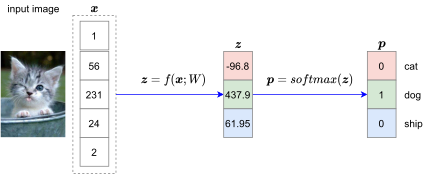
Score function
The score function f that maps the raw features to class scores. \boldsymbol{z}=f(\boldsymbol{x};{\color{red}W},{\color{red}\boldsymbol{b}})={\color{red}W}\boldsymbol{x}+{\color{red}\boldsymbol{b}}
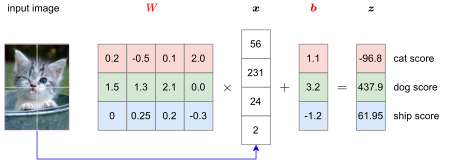
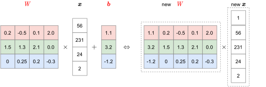
- Use bias trick {\color{red}W_{0}}={\color{red}\boldsymbol{b}} to represent the two parameters {\color{red}W},{\color{red}\boldsymbol{b}} as one \boldsymbol{z}=f(\boldsymbol{x};{\color{red}W})={\color{red}W}\boldsymbol{x}
Softmax function
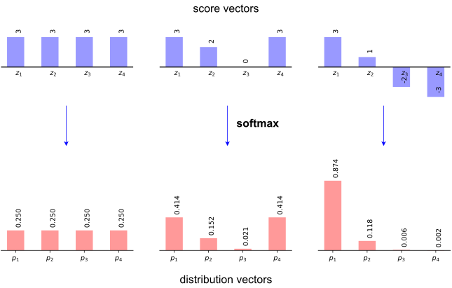
The softmax function converts a score vector \boldsymbol{z}=(z_{1},...,z_{C}) to a discrete distribution vector \boldsymbol{p}=(p_{1},...,p_{C}) p_{i}=P(y=i\mid\boldsymbol{z})=\phi_{i}(\boldsymbol{z})=\frac{e^{z_{i}}}{\sum_{j=1}^{C}e^{z_{j}}},\;i\in[1,...,C] where z_{i}={\color{red}w}_{{\color{red}i0}}+{\color{red}w}_{{\color{red}i1}}x_{1}+...+{\color{red}w}_{{\color{red}iD}}x_{D}={\color{red}\boldsymbol{w}}_{{\color{red}i}}^{\mathbin{\color{red}\intercal}}\boldsymbol{x}
Problem Statement
Given \mathcal{D}=\{(\boldsymbol{x}_{1},y_{1})...(\boldsymbol{x}_{N},y_{N})\} where y_{n}\in\{1,...,C\}.
Denote \boldsymbol{t}_{n} is a one-hot encoding of y_{n} (or target discrete distribution)
Learning goal: Find a softmax function \boldsymbol{\phi}_{{\color{red}W}}(\cdot)=\{\phi_{1},...,\phi_{C}\} that minimize \arg\min_{{\color{red}W}}E(\boldsymbol{\phi}_{{\color{red}W}})=\arg\min_{{\color{red}W}}\sum_{n=1}^{N}CE(\boldsymbol{p}_{n},\boldsymbol{t}_{n})
Cross Entropy
Cross-entropy (CE) is a measure of the difference between two probability distributions. The cross-entropy between a “true” distribution \boldsymbol{t}=(t_{1},...,t_{C}) and an estimated distribution \boldsymbol{p}=(p_{1},...,p_{C}) is defined as CE(\boldsymbol{p},\boldsymbol{t})=-\sum_{i=1}^{C}t_{i}\log p_{i}
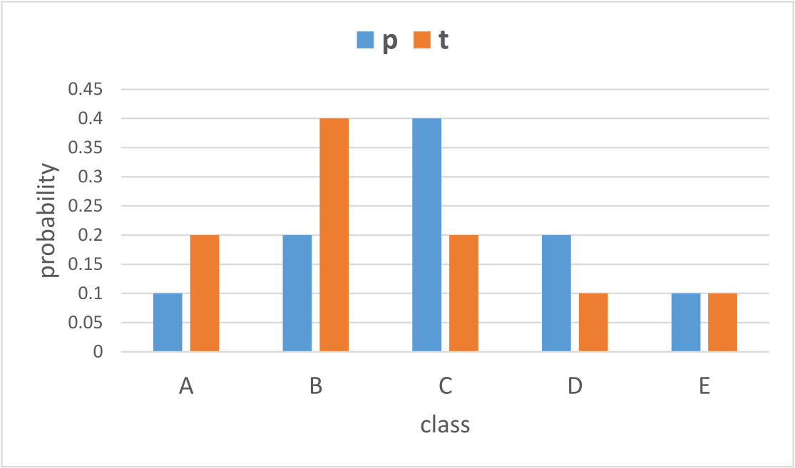
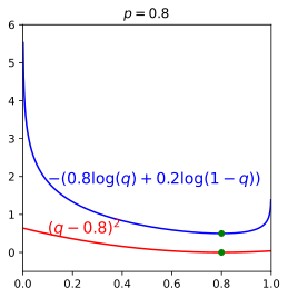
\left.\begin{array}{c} \boldsymbol{p}=(0.1,0.2,0.4,0.2,0.1)\\ \boldsymbol{t}=(0.2,0.4,0.2,0.1,0.1) \end{array}\right\} \to CE(\boldsymbol{p},\boldsymbol{t})=1.678
CE>0
CE(\boldsymbol{p},\boldsymbol{t})\neq CE(\boldsymbol{t},\boldsymbol{p})
CE minimize if p_{i}=t_{i},\forall i
MSE
Mean squared error (MSE) is a measure of the average of the squares of the errors. MSE(\boldsymbol{p},\boldsymbol{t})=\frac{1}{C}\sum_{i=1}^{C}(p_{i}-t_{i})^{2}
MSE\geq0
MSE(\boldsymbol{p},\boldsymbol{t})=MSE(\boldsymbol{t},\boldsymbol{p})
MSE=0 if p_{i}=t_{i},\forall i
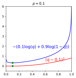
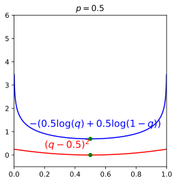
Cross Entropy vs. MSE
- Consider three “true” binary distributions \boldsymbol{p}=(0.1,0.9),(0.5,0.5) and (0.8,0.2)
Learning Algorithm
Initialize the weights {\color{red}W}_{0} (parameters) at t=0
For t=1,2,3,... do
Compute the ouput distribution \boldsymbol{p}_{n} for each \boldsymbol{x}_{n} (n=1...N) \begin{equation} \boldsymbol{p}_{n}=softmax({\color{red}W}_{t}\boldsymbol{x}_{n}) \end{equation}
Compute the gradient \begin{equation} \nabla_{{\color{red}W}}E=\frac{1}{N}\sum_{n=1}^{N}(\boldsymbol{p}_{n}-\boldsymbol{t}_{n})\boldsymbol{x}_{n}^{\intercal} \end{equation}
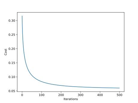
Update the weights \begin{equation} {\color{red}{\color{red}W}}_{t+1}={\color{red}W}_{t}-{\color{green}\eta}\nabla_{{\color{red}W}}E \end{equation}
Iterate the next step until {\color{red}W} is not change
Return the final weights {\color{red}W}
Example
- Softmax regression for Iris dataset
3.7 Capacity, Overfitting and Underfitting
Model Capacity
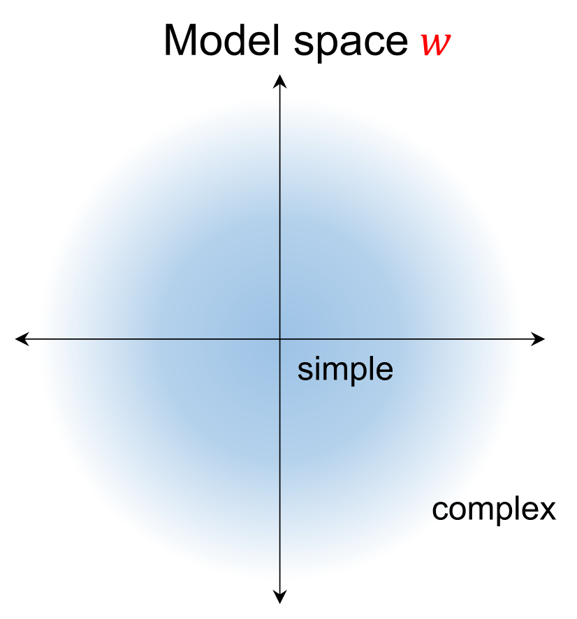
Capacity is model complexity.
The most common ways to estimate the capacity of a model:
VC dimension
The number of parameters
The norm of parameters
Model vs. Data
Data is divided into three sets: training set, validation set and test set.
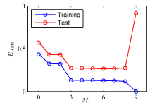
Models can be too limited. We can’t find a function that fits the data well. This is called underfitting.
Models can also be too rich. We don’t just model the data, but also the underlying noise. This is called overfitting.
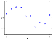
Given the data set \mathcal{D}=\{(x_{1},y_{1}),...(x_{10},y_{10})\} shown in the following figure, find the best regression function to the data
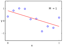
Consider the simple hypothesis set \mathcal{H}_{1}=\{h\mid y=h(x)={\color{red}w_{0}}+{\color{red}w}_{{\color{red}1}}x\}
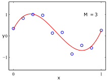
Consider the hypothesis set \mathcal{H}_{3}=\{h\mid y=h(x)={\color{red}w_{0}}+{\color{red}w}_{{\color{red}1}}x+{\color{red}w_{2}}x^{2}+{\color{red}w}_{{\color{red}3}}x^{3}\} (note that \mathcal{H}_{1}\subset\mathcal{H}_{3})
Consider the hypothesis set \mathcal{H}_{9}=\{h\mid y=h(x)={\color{red}w}_{{\color{red}0}}+{\color{red}w}_{{\color{red}1}}x+{\color{red}w}_{{\color{red}2}}x^{2}+...+{\color{red}w}_{{\color{red}9}}x^{9}\} (note that \mathcal{H}_{1}\subset\mathcal{H}_{3}\subset\mathcal{H}_{9})
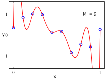
Which one
Under-fitting
Over-fitting
Appropriate fitting
| M=1 | M=3 | M=9 | |
|---|---|---|---|
| {\color{red}w_{0}} | 0.82 | 0.31 | 0.35 |
| {\color{red}w_{1}} | -1.27 | 7.99 | 232.37 |
| {\color{red}w_{2}} | -25.43 | -5321.83 | |
| {\color{red}w_{3}} | 17.37 | 48568.31 | |
| {\color{red}w_{4}} | -231639.30 | ||
| {\color{red}w_{5}} | 640042.26 | ||
| {\color{red}w_{6}} | -1061800.52 | ||
| {\color{red}w_{7}} | 1042400.18 | ||
| {\color{red}w_{8}} | -557682.99 | ||
| {\color{red}w_{9}} | 125201.43 |
Model Performance
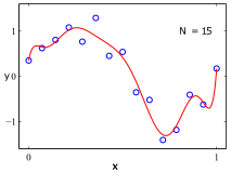
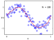
What happen if increasing N
Errors in Learning Model
Bias errors: error due to assumption in the model
- High bias to signify underfitting
Variance errors: It measures the variability in the results given by model when the dataset is changed
- High variance to signify overfitting
\text{Expected error}=\text{Bias}+\text{Variance}+\text{Irreducible Error}
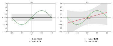
Given a learning model \left\langle \mathcal{H},\mathcal{A}\right\rangle, we define the “average” hypothesis \overline{g}(x) \overline{g}(x)=\mathbb{E}_{\mathcal{D}}\left[g_{\mathcal{D}}(x)\right] where g_{\mathcal{D}}(x) is the “best” hypothesis given the data set \mathcal{D}
Bias of learning model \text{Bias}=\mathbb{E}_{x}\left[\left(\overline{g}(x)-f(x)\right)^{2}\right] where f(x) is the “truth” function
Variance of learning model \text{Variance}=\mathbb{E}_{x}\left[\mathbb{E}_{\mathcal{D}}\left[(g_{\mathcal{D}}(x)-\overline{g}(x))^{2}\right]\right]
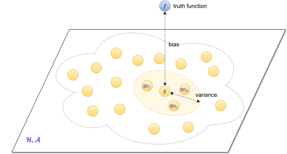
- Given many independent data sets \mathcal{D}_{1},\mathcal{D}_{2},...,\mathcal{D}_{K}, we can estimate \overline{g}(x) by \overline{g}(x)\approx\frac{1}{K}\sum_{i=1}^{K}g_{\mathcal{D}_{i}}(x)
Example: two learning models
Consider a target function sine \begin{array}{llccc} f & : & [-1,1] & \to & \mathbb{R}\\ & & x & \to & \sin(\pi x) \end{array}
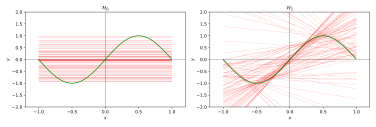
We generate 100 data sets \left\{ \mathcal{D}_{i}\right\} ,i=1,...,100, each containing N=2 data points, independently from the sinusoidal curve f(x)=\sin(\pi x). For each data set \mathcal{D}_{i}, we fit the data using one of two models
\mathcal{H}_{0}: set of all lines of the form h(x)={\color{red}b}
\mathcal{H}_{1}: set of all lines of the form h(x)={\color{red}a}x+{\color{red}b}
Note that \mathcal{H}_{0}\subset\mathcal{H}_{1}
Given a data set \mathcal{D}_{i}=\{(x_{1},y_{1}),(x_{2},y_{2})\}.
For \mathcal{H}_{0}, we choose the constant hypothesis that best fits the data (the horizontal line at the midpoint, b=(y_{1}+y_{2})/2).
For \mathcal{H}_{1}, we choose the line that passes through the two data points (x_{1},y_{1}) and (x_{2},y_{2}).
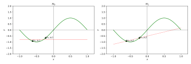
Repeating this process with 100 data sets \left\{ \mathcal{D}_{i}\right\} ,i=1,...,100,
The bias-variance for each learning model
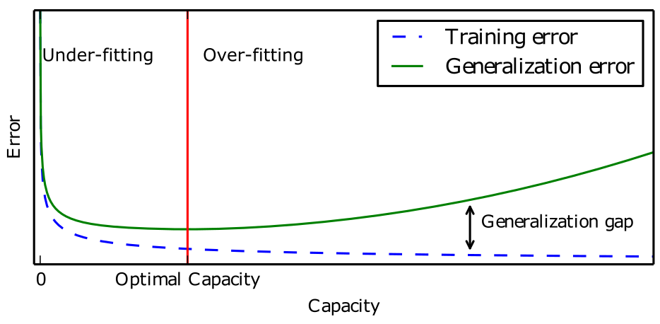
Generalization and Capacity
The criteria determining how well a machine learning model will perform:
Make the training error small.
Make the gap between training and test (generalization) error small.
Regularization
Regularization is any modification we make to a learning model that is intended to reduce its generalization error but not its training error.
Addressing
| High bias | High variance |
|---|---|
| Obtain more features | Decrease number of features |
| Decrease regularization {\color{green}\lambda} | Increase regularization {\color{green}\lambda} |
| Extend model | Obtain more data |
| Train longer | Stop early |
| New model architecture | New model architecture |
Regularization for Linear Regression
Using regularized MSE_{train} for linear regression \boldsymbol{{\color{red}w}}=\arg\min_{\boldsymbol{{\color{red}w}}}\left[MSE_{train}+{\color{green}\lambda}\left(\frac{1}{N}\boldsymbol{{\color{red}w}}^{T}\boldsymbol{{\color{red}w}}\right)\right] where {\color{green}\lambda} is the regularization coefficient (hyper-parameter) that controls the relative importance of the data-dependent error MSE_{train} and the regularization term {\color{green}\lambda}\left(\frac{1}{N}\boldsymbol{{\color{red}w}}^{T}\boldsymbol{{\color{red}w}}\right)
Solving for \boldsymbol{{\color{red}w}}, we obtain \boldsymbol{{\color{red}w}}=(\boldsymbol{X}^{\intercal}\boldsymbol{X}+{\color{green}\lambda}\boldsymbol{I})^{-1}\boldsymbol{X}^{\intercal}\boldsymbol{y}
Tradeoff of Regularization
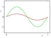
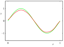
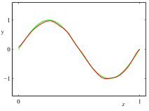
Example: one learning model
Consider a target function sine \begin{array}{llccc} f & : & [-1,1] & \to & \mathbb{R}\\ & & x & \to & \sin(2\pi x) \end{array}
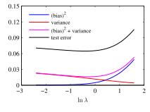
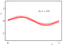
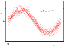
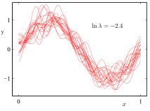
We generate 100 data sets \left\{ \mathcal{D}_{i}\right\} ,i=1,...,100, each containing N=25 data points, independently from the sinusoidal curve f(x)=\sin(2\pi x). For each data set \mathcal{D}_{i}, we fit a model with 24 Gaussian basis functions by minimizing the regularized error function
Illustration of the dependence of bias and variance on model regularization coefficient
Summary of the dependence of bias and variance on model regularization coefficient