16 SEQUENCE MODELS
16.1 Sequential prediction tasks
Recurrent Neural Networks: Process Sequences
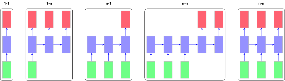
Model 1-1: e.g. Image classification
Model 1-n: e.g. Image captioning
Model n-1: e.g. Sentiment classification
Model n-n: e.g. Machine translation
Model n-n: e.g. Intellisense
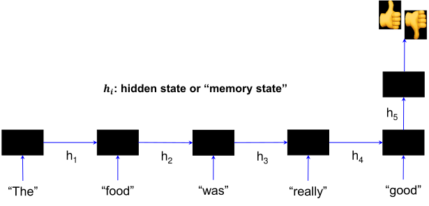
Example 1: Sentiment classification
- Goal: classify a text sequence (e.g., restaurant, movie or product review, Tweet) as having positive or negative sentiment
“The food was really good”
“The vacuum cleaner broke within two weeks”
“The movie had slow parts, but overall was worth watching”
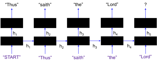
Example 2: Text generation
- Goal: Sample from the distribution of a given text corpus (also known as language modeling)
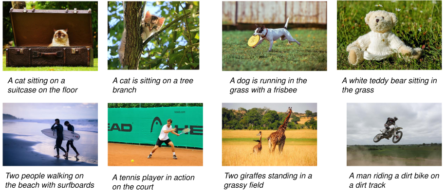
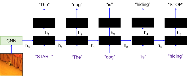
Example 3: Image caption generation
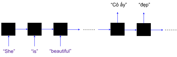
Example 4: Machine translation
- Translate English to Vietnamese
16.2 Recurrent Network Network
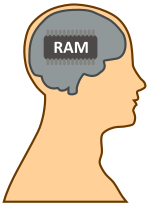
Human thoughts are persistence
- Humans don’t start their thinking from scratch. They usually use their prior knowledge or experiences.
Architecture
Recurrent Neural Network
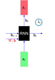
- Key idea: RNNs have an “internal state” h_{t} that is updated as a sequence is processed
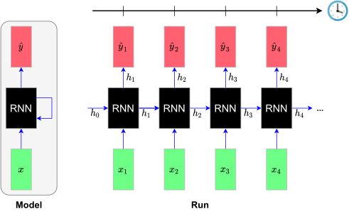
Vanilla RNN unit
- The state consists of a single “hidden” vector \boldsymbol{h}_{t}:
Full formula
\begin{equation} \begin{array}{l} \left\{ \begin{array}{l} \boldsymbol{h}_{t}=f_{{\color{red}W,\boldsymbol{b}}}(\boldsymbol{h}_{t-1},\boldsymbol{x}_{t})\\ \hat{\boldsymbol{y}}_{t}=g_{{\color{red}W,\boldsymbol{b}}}(\boldsymbol{h}_{t}) \end{array}\right.\\ \left\{ \begin{array}{l} \boldsymbol{h}_{t}=\tanh({\color{red}W}_{hh}\boldsymbol{h}_{t-1}+{\color{red}W}_{xh}\boldsymbol{x}_{t}+\boldsymbol{{\color{red}b}}_{h})\\ \hat{\boldsymbol{y}}_{t}={\color{red}W}_{hy}\boldsymbol{h}_{t}+\boldsymbol{{\color{red}b}}_{y} \end{array}\right. \end{array} \end{equation} where parameters {\color{red}W}=({\color{red}W}_{xh},{\color{red}W}_{hh},{\color{red}W}_{hy}) and {\color{red}\boldsymbol{b}}=(\boldsymbol{{\color{red}b}}_{h},\boldsymbol{{\color{red}b}}_{y})
Simple formula without bias vector
\begin{equation} \begin{array}{l} \left\{ \begin{array}{l} \boldsymbol{h}_{t}=\tanh({\color{red}W}_{hh}\boldsymbol{h}_{t-1}+{\color{red}W}_{xh}\boldsymbol{x}_{t})\\ \hat{\boldsymbol{y}}_{t}={\color{red}W}_{hy}\boldsymbol{h}_{t} \end{array}\right.\end{array} \end{equation}
Training
Cost function
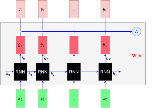
- Given a sequence \{(x_{1,}y_{1}),...,(x_{T},y_{T})\}, the lost function L is defined by \begin{equation} L(x_{1},\ldots,x_{T},y_{1},\ldots,y_{T}\mid{\color{red}W},{\color{red}\boldsymbol{b}})=\sum_{t=1}^{T}l(y_{t},\hat{y}_{t}) \end{equation}
RNN forward
Given a sequence data\{(\boldsymbol{x}_{1,}\boldsymbol{y}_{1}),...,(\boldsymbol{x}_{T},\boldsymbol{y}_{T})\}
For each t=1...T, compute using simple formula \left\{ \begin{array}{l} \boldsymbol{h}_{t}=\tanh({\color{red}W}_{hh}\boldsymbol{h}_{t-1}+{\color{red}W}_{xh}\boldsymbol{x}_{t})\\ \hat{\boldsymbol{y}}_{t}={\color{red}W}_{hy}\boldsymbol{h}_{t} \end{array}\right.
Compute the lost function L(\boldsymbol{x}_{1},\ldots,\boldsymbol{x}_{T},\boldsymbol{y}_{1},\ldots,\boldsymbol{y}_{T}\mid{\color{red}W})=\sum_{t=1}^{T}l(\boldsymbol{y}_{t},\hat{\boldsymbol{y}}_{t})
RNN backward
- For each RNN unit
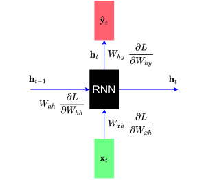
\begin{equation} \begin{array}{rcl} \dfrac{\partial L}{\partial{\color{red}W}_{hh}} & = & \dfrac{\partial L}{\partial\boldsymbol{h}_{t}}\odot(1-\tanh^{2}({\color{red}W}_{hh}\boldsymbol{h}_{t-1}+{\color{red}W}_{xh}\boldsymbol{x}_{t}))\boldsymbol{h}_{t-1}^{\intercal}\\ \dfrac{\partial L}{\partial{\color{red}W}_{xh}} & = & \dfrac{\partial L}{\partial\boldsymbol{h}_{t}}\odot(1-\tanh^{2}({\color{red}W}_{hh}\boldsymbol{h}_{t-1}+{\color{red}W}_{xh}\boldsymbol{x}_{t}))\boldsymbol{x}_{t}^{\intercal}\\ \dfrac{\partial L}{\partial{\color{red}W}_{hy}} & = & ?\\ \dfrac{\partial L}{\partial\boldsymbol{h}_{t-1}} & = & {\color{red}W}_{hh}^{\intercal}(1-\tanh^{2}({\color{red}W}_{hh}\boldsymbol{h}_{t-1}+{\color{red}W}_{xh}\boldsymbol{x}_{t}))\odot\dfrac{\partial L}{\partial\boldsymbol{h}_{t}} \end{array} \end{equation}
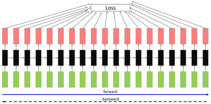
Backpropagation through time (BPTT)
- Problem: Takes a lot of memory for long sequences!
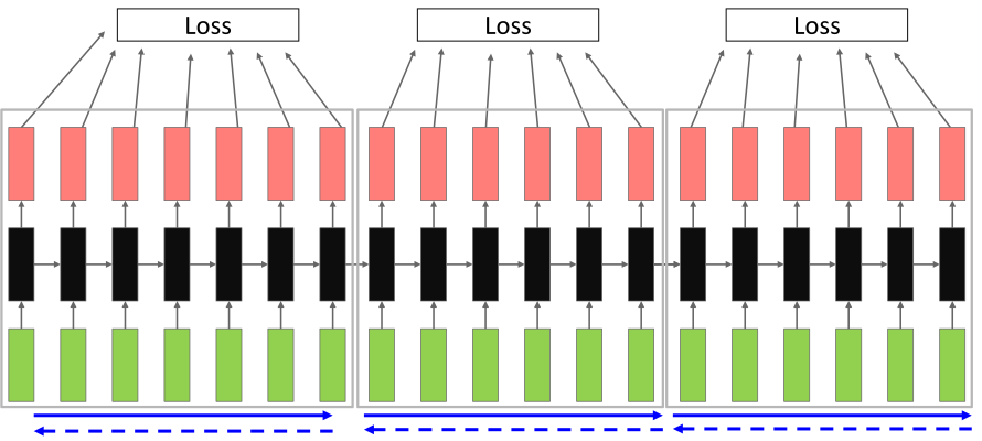
Truncated backpropagation through time
- In practice, truncated BPTT is used: run the RNN forward k time steps, propagate backward for k time steps
Learning problems
Long-term dependencies
Vanilla RNNs trained with BPTT have difficulties learning long-term dependencies.
Able when the gap between the relevant information is small.
As that gap grows, unable to learn to connect the information.

Vanishing/Exploding gradients
Computing gradient of h_{0} involves many factors of {\color{red}W} (and repeated tanh)
Largest singular value >1: Exploding gradients
Gradient clipping: Scale gradient \boldsymbol{g} if its norm is too big \begin{equation} \boldsymbol{g}\leftarrow\min\left(1,\frac{\text{threshold}}{\|\boldsymbol{g}\|}\right)\boldsymbol{g} \end{equation}
Largest singular value <1: Vanishing gradients
Change RNN architecture
16.3 Modern Recurrent Neural Networks
Long Short Term Memory (LSTM)
Key Concepts
Maintain a separate cell state c_{t} from what is outputted
Use gates to control the flow of information
Forget gate gets rid of irrelevant information
Selectively update cell state
Output gate returns a filtered version of the cell state
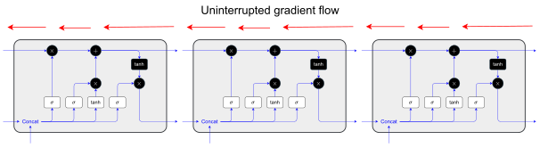
Backpropagation from c_{t} to c_{t-1} doesn’t require matrix multiplication \to avoid vanishing gradient problem (uninterrupted gradient flow)
Long Short Term Memory Unit
{\color{red}i} (input gate): Whether to write to cell?
{\color{red}f} (forget gate): Whether to erase cell?
{\color{red}o} (output gate): How much to reveal cell?
{\color{red}g} (candiate gate): How much to write to cell?
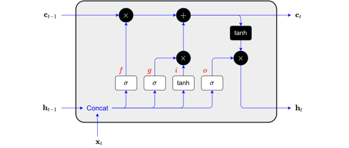
\begin{align} \left(\begin{array}{c} \boldsymbol{i}_{t}\\ \boldsymbol{f}_{t}\\ \boldsymbol{o}_{t}\\ \boldsymbol{g}_{t} \end{array}\right) & =\left(\begin{array}{c} \sigma\\ \sigma\\ \sigma\\ \tanh \end{array}\right)\left({\color{red}W}\left(\begin{array}{c} \boldsymbol{h}_{t-1}\\ \boldsymbol{x}_{t} \end{array}\right)+{\color{red}\boldsymbol{b}}_{h}\right)\\ \boldsymbol{c}_{t} & =\boldsymbol{f}_{t}\odot\boldsymbol{c}_{t-1}+\boldsymbol{i}_{t}\odot\boldsymbol{g}_{t}\nonumber \\ \boldsymbol{h}_{t} & =\boldsymbol{o}_{t}\odot\tanh(\boldsymbol{c}_{t})\nonumber \end{align}
Gradient flow
- Similar to ResNet
Gated Recurrent Units (GRU)
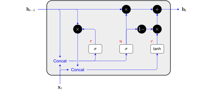
GRU: Key Concepts
GRUs get rid of separate cell states; only use:
Reset gates {\color{red}r} help capture short-term dependencies in sequences.
Update gates {\color{red}u} help capture long-term dependencies in sequences.
Candiate gates {\color{red}c}
Deep Recurrent Neural Networks
Deep Recurrent Neural Networks
- Multilayer LSTMs
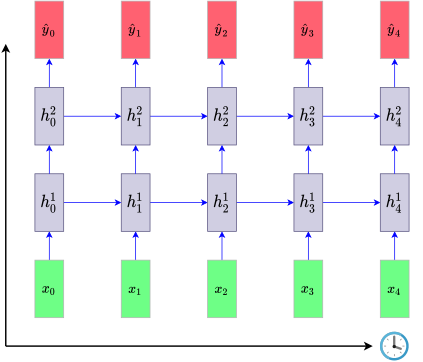
\begin{align*} \left(\begin{array}{c} \boldsymbol{i}_{t}^{\ell}\\ \boldsymbol{f}_{t}^{\ell}\\ \boldsymbol{o}_{t}^{\ell}\\ \boldsymbol{g}_{t}^{\ell} \end{array}\right) & =\left(\begin{array}{c} \sigma\\ \sigma\\ \sigma\\ \tanh \end{array}\right)\left({\color{red}W}\left(\begin{array}{c} \boldsymbol{h}_{t-1}^{\ell}\\ \boldsymbol{h}_{t}^{\ell-1} \end{array}\right)+{\color{red}\boldsymbol{b}}_{h}^{\ell}\right)\\ \boldsymbol{c}_{t}^{\ell} & =\boldsymbol{f}_{t}^{\ell}\odot\boldsymbol{c}_{t-1}^{\ell}+\boldsymbol{i}_{t}^{\ell}\odot\boldsymbol{g}_{t}^{\ell}\\ \boldsymbol{h}_{t}^{\ell} & =\boldsymbol{o}_{t}^{\ell}\odot\tanh(\boldsymbol{c}_{t}^{\ell}) \end{align*}
BidirectionalRecurrent Neural Networks
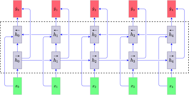
Bidirectional Model
- Bidirectional RNNs add a hidden layer that passes information in a backward direction
Encoder-Decoder Architecture
Encoder-Decoder Architecture
A encoder-decoder architecture includes two major components
The first component is an encoder: it takes a variable-length sequence as the input and transforms it into a state with a fixed shape.
The second component is a decoder: it maps the encoded state of a fixed shape to a variable-length sequence.
