5 INSTANCE BASED LEARNING

Parametric vs Non-parametric Models

Parametric Models

In the models that we have seen, we select a hypothesis space \mathcal{H} and adjust a fixed set of parameters \boldsymbol{{\color{red}w}} with the training data \mathcal{D}
We assume that the parameters \boldsymbol{{\color{red}w}} summarize the training data \mathcal{D} and we can forget about it

Non-parametric Models

A non parametric model is one that can not be characterized by a fixed set of parameters
A family of non parametric models is Instance Based Learning. The function is based on the training data \mathcal{D}=\{\boldsymbol{x}_{1},\boldsymbol{x}_{2},...\boldsymbol{x}_{n}\}

\begin{equation} y=f(\boldsymbol{x};{\color{red}\boldsymbol{w}}) \end{equation}

\begin{equation} y=f(\boldsymbol{x};\boldsymbol{x}_{1},\boldsymbol{x}_{2},...,\boldsymbol{x}_{n}) \end{equation}

Inductive Bias

In nonparametric model, we assume that similar inputs have similar outputs.

This is a reasonable assumption: The world is smooth, and functions, whether they are densities, discriminants, or regression functions, change slowly. Similar instances mean similar things.

5.1 Classification

k-Nearest Neighbor (k-NN)

When To Consider Nearest Neighbor

Data points \boldsymbol{x}\in\mathbb{R}^{D}
Less than D<20 attributes
Lots of training data \mathcal{D}

Nearest Neighbor

Learning mode

Store all training examples \mathcal{D}=\{(\boldsymbol{x}_{i},y_{i})\mid i=1,...,N\}

Running mode

Nearest neighbor: Given query instance \boldsymbol{x}_{q}, first locate the nearest neighbhor \boldsymbol{x}^{(1)}, then estimate \begin{equation} h(\boldsymbol{x}_{q})=y^{(1)} \end{equation}
{\color{green}k}-Nearest neighbor: Given \boldsymbol{x}_{q}, take vote among its {\color{green}k} nearest neighbors \{\boldsymbol{x}^{(1)},\boldsymbol{x}^{(2)},...,\boldsymbol{x}^{({\color{green}k})}\} \begin{equation} h(\boldsymbol{x}_{q})=\text{majority vote}\{y^{(1)},y^{(2)},...,y^{({\color{green}k})}\} \end{equation}

Distance

Some common distances in space \mathbb{R}^{D}

The Minkowski distance of order p>0 \begin{equation} d(\boldsymbol{x},\boldsymbol{y})=L_{p}(\boldsymbol{x},\boldsymbol{y})=\left(\sum_{i=1}^{D}|x_{i}-y_{i}|^{p}\right)^{1/p} \end{equation}
Euclidean distance (popular) \begin{equation} d(\boldsymbol{x},\boldsymbol{y})=L_{2}(\boldsymbol{x},\boldsymbol{y})=\sqrt{\sum_{i=1}^{D}(x_{i}-y_{i})^{2}} \end{equation}
Manhattan distance \begin{equation} d(\boldsymbol{x},\boldsymbol{y})=L_{1}(\boldsymbol{x},\boldsymbol{y})=\sum_{i=1}^{D}|x_{i}-y_{i}| \end{equation}
Contours of the distance from the origin O for various values of the parameter p

The Curse of dimensionality

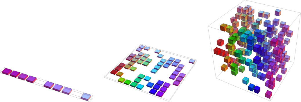
The more dimensions we have, the more examples we need
The number of examples that we have in a volume of space decreases exponentially with the number of dimensions
- If the number of dimensions is very high, the nearest neighbours can be very far away

Analysis

Advantages

No training, just store data
Learn complex target functions
Don’t lose information

Disadvantages

Slow at query time
Easily fooled by irrelevant attributes

Effects of Hyper-parameters

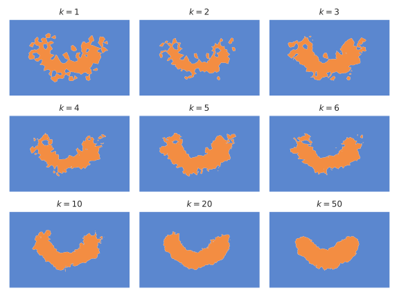
Parameter k

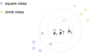
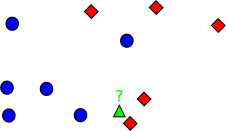
if k=1 the cross point \boldsymbol{x} should be classified to square class
if k=3 ?
if k=5 ?
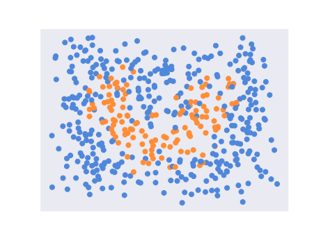
Data set \mathcal{D} with 500 samples belonging to two classes {blue, orange}
Decision regions for various values of {\color{green}k}

5.2 Metric Learning

Motivation

Nearest neighbor classification
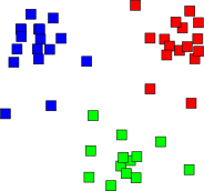
Clustering
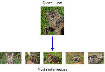
Information retrieval
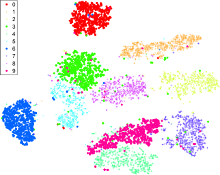
Data visualization

Metric Learning

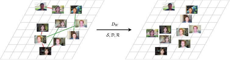
Given a set of data points \mathcal{X} and their corresponding labels \mathcal{Y}
Select a parametric distance or similarity function \begin{equation} d_{{\color{red}W}}(\boldsymbol{x},\boldsymbol{x}')=L\left(f_{{\color{red}W}}(\boldsymbol{x}),f_{{\color{red}W}}(\boldsymbol{x}')\right) \end{equation}
- An embedding function (parametric function) \begin{equation} f_{{\color{red}W}}(\boldsymbol{x})\colon\mathcal{X}\to\mathbb{R}^{n} \end{equation}
- A distance function (which is usually fixed beforehand) \begin{equation} L(\boldsymbol{x},\boldsymbol{x}')\colon\mathbb{R}^{n}\times\mathbb{R}^{n}\to\mathbb{R} \end{equation}
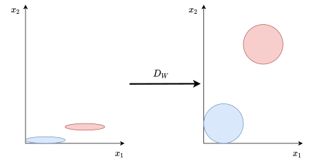
The goal is to train the parametric distance, so that the combination d_{{\color{red}W}}(\boldsymbol{x},\boldsymbol{x}') produces small values if the labels y,y'\in\mathcal{Y} of the samples \boldsymbol{x},\boldsymbol{x}'\in\mathcal{X} are equal, and larger values if they aren’t.
Collect similarity judgements on data pairs/triplets \begin{align} \mathcal{S} & = & \{(\boldsymbol{x}_{i},\boldsymbol{x}_{j}):\boldsymbol{x}_{i}\text{ and }\boldsymbol{x}_{j}\text{ should be similar}\},\nonumber \\ \mathcal{D} & = & \{(\boldsymbol{x}_{i},\boldsymbol{x}_{j}):\boldsymbol{x}_{i}\text{ and }\boldsymbol{x}_{j}\text{ should be dissimilar}\}.\\ \mathcal{R} & = & \{(\boldsymbol{x}_{i},\boldsymbol{x}_{j},\boldsymbol{x}_{k}):\boldsymbol{x}_{i}\text{ should be more similar to }\boldsymbol{x}_{j}\text{ than to }\boldsymbol{x}_{k}\}.\nonumber \end{align}
Estimate parameters s.t. metric best agrees with judgements \begin{equation} \hat{{\color{red}W}}=\begin{aligned}\arg\min_{{\color{red}W}} & \left[\underset{\text{loss function}}{\underbrace{\ell(d_{{\color{red}W}},\mathcal{S},\mathcal{D},\mathcal{R})}}+\underset{\text{regularization}}{\underbrace{\lambda R({\color{red}W})}}\right]\end{aligned} \end{equation}

Contrastive Approaches

An embedding function is usually a neural network
A distance function is L_{2} distance
A loss function

Loss Function

Contrastive Loss

Contrastive Loss (Chopra et al. 2005)

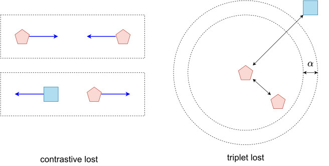
Let \boldsymbol{x}_{1},\boldsymbol{x}_{2} be some samples in the dataset, and y_{1},y_{2} are their corresponding labels. Also, for some condition A, let’s denote \mathbb{I}{}_{A} as the identity function that is equal to 1 if A is true, and 0 otherwise. The loss function is then defined as follows: \begin{align} \ell_{\text{contrast}} & =\mathbb{I}_{y_{1}=y_{2}}d_{{\color{red}W}}(\boldsymbol{x}_{1},\boldsymbol{x}_{2})+\mathbb{I}_{y_{1}\ne y_{2}}\max\left(0,\alpha-d_{{\color{red}W}}(\boldsymbol{x}_{1},\boldsymbol{x}_{2})\right) \end{align} where \alpha is the margin.

Triplet Loss

Triplet Loss (Schroff et al. 2015)

Let \boldsymbol{x}_{a},\boldsymbol{x}_{p},\boldsymbol{x}_{n} be some samples from the dataset and \boldsymbol{y}_{a},\boldsymbol{y}_{p},\boldsymbol{y}_{n} be their corresponding labels, so that y_{a}=y_{p} and y_{a}\ne y_{n}. Usually, \boldsymbol{x}_{a} is called anchor sample, \boldsymbol{x}_{p} is called positive sample because it has the same label as \boldsymbol{x}_{a}, and \boldsymbol{x}_{n} is called negative sample because it has a different label. It is defined as: \begin{align} \ell_{\text{triplet}} & =\max\left(0,d_{{\color{red}W}}(\boldsymbol{x}_{a},\boldsymbol{x}_{p})-d_{{\color{red}W}}(\boldsymbol{x}_{a},\boldsymbol{x}_{n})+\alpha\right) \end{align} where \alpha is the margin.

Contrastive Loss vs. Triplet Loss

5.3 Regression

Feature Space

Project the data into a higher dimensional space (feature space) \mathcal{F}

Transformation function

\begin{equation} \begin{array}{ccccc} \phi & : & \mathbb{R}^{D} & \to & \mathcal{F}\\ & & \boldsymbol{x}_{i} & \to & \phi(\boldsymbol{x}_{i}) \end{array} \end{equation}

Work with \phi(\boldsymbol{x}_{i}) instead of working with \boldsymbol{x}_{i}.

Kernel Function

The Kernel Function

A kernel is a function k(\boldsymbol{x},\boldsymbol{z}) which represents a dot product in a “hidden” feature space of \phi. \begin{equation} k(\boldsymbol{x},\boldsymbol{z})=\phi(\boldsymbol{x})\cdot\phi(\boldsymbol{z}) \end{equation}

Note that: we have only dot products \phi(\boldsymbol{x}_{i})\cdot\phi(\boldsymbol{x}_{j}) to compute; however, this could be very expensive in a high dimensional space.
Kernel trick:

instead of \phi(\boldsymbol{x})=\phi\left(\begin{array}{c} x_{1}\\ x_{2} \end{array}\right)=\left(\begin{array}{c} x_{1}^{2}\\ \sqrt{2}x_{1}x_{2}\\ x_{2}^{2} \end{array}\right), use k(\boldsymbol{x},\boldsymbol{z})=(\boldsymbol{x}\cdot\boldsymbol{z})^{2}

Common Kernels

Polynomial: \begin{equation} k(\boldsymbol{x},\boldsymbol{z})=(u\boldsymbol{x}\cdot\boldsymbol{z}+v)^{p}\;(u\in\mathbb{R},v\in\mathbb{R},p\in\mathbb{N}) \end{equation}
Gaussian: \begin{equation} k(\boldsymbol{x},\boldsymbol{z})=\exp\left(-\frac{\left\Vert \boldsymbol{x}-\boldsymbol{z}\right\Vert ^{2}}{{\color{green}\sigma}^{2}}\right)\;,{\color{green}\sigma}\in\mathbb{R}^{+} \end{equation} Note: feature space is infinite-dimensional

Techniques for Construction of Kernels

In all the following, k_{1},k_{2},...,k_{j} are assumed to be valid kernel functions

Scalar multiplication: The validity of a kernel is conserved after multiplication by a positive scalar, i.e., for any \alpha>0, the function \begin{equation} k(\boldsymbol{x},\boldsymbol{z})=\alpha k_{1}(\boldsymbol{x},\boldsymbol{z}) \end{equation}
Adding a positive constant: For any positive constant \alpha>0, the function \begin{equation} k(\boldsymbol{x},\boldsymbol{z})=\alpha+k_{1}(\boldsymbol{x},\boldsymbol{z}) \end{equation}
Linear combination: A linear combination of kernel functions involving only positive weights, i.e., \begin{equation} k(\boldsymbol{x},\boldsymbol{z})=\sum_{j=1}^{m}\alpha_{j}k_{j}(\boldsymbol{x},\boldsymbol{z}),\qquad\text{with }\alpha_{j}>0 \end{equation} is a valid kernel function.
Product: The product of two kernel functions, i.e., \begin{equation} k(\boldsymbol{x},\boldsymbol{z})=k_{1}(\boldsymbol{x},\boldsymbol{z})k_{2}(\boldsymbol{x},\boldsymbol{z}) \end{equation} is a valid kernel function.
Polynomial functions of a kernel output: Given a polynomial f:\mathbb{R}\to\mathbb{R} with positive coefficients, the function \begin{equation} k(\boldsymbol{x},\boldsymbol{z})=f(k_{1}(\boldsymbol{x},\boldsymbol{z})) \end{equation} is a valid kernel function.
Exponential function of a kernel output: The function \begin{equation} k(\boldsymbol{x},\boldsymbol{z})=\exp(k_{1}(\boldsymbol{x},\boldsymbol{z})) \end{equation} is a valid kernel function.
Product of matrix and vectors: \begin{equation} k(\boldsymbol{x},\boldsymbol{z})=\boldsymbol{x}^{\intercal}A\boldsymbol{z} \end{equation} where A is a symmetric positive semidefinite matrix.

Kernel Regression

Linear Regression Revisted

Problem: Given a dataset of input-output pairs \mathcal{D}=\{(\boldsymbol{x}_{1},y_{1}),\ldots,(\boldsymbol{x}_{N},y_{N})\}, find the best linear regresion

Primal form \begin{equation} \hat{y}=f(\boldsymbol{x})=\sum_{i=1}^{D}{\color{red}w_{i}}x_{i} \end{equation} where \begin{equation} \boldsymbol{{\color{red}w}}=(\boldsymbol{X}^{\intercal}\boldsymbol{X}+{\color{green}\lambda}\boldsymbol{I}_{D})^{-1}\boldsymbol{X}^{\intercal}\boldsymbol{y} \end{equation}
Dual Form \begin{equation} \hat{y}=f(\boldsymbol{x})=\sum_{i=1}^{N}{\color{red}\alpha_{i}}\boldsymbol{x}_{i}^{\intercal}\boldsymbol{x} \end{equation} where \begin{equation} \boldsymbol{{\color{red}\alpha}}=(\boldsymbol{X}\boldsymbol{X}^{\intercal}+{\color{green}\lambda}\boldsymbol{I}_{N})^{-1}\boldsymbol{y} \end{equation}

The Kernel Trick

Question: How introduce nonlinearity to \hat{y}=f(\boldsymbol{x})=\sum_{i=1}^{N}{\color{red}\alpha_{i}}\boldsymbol{x}_{i}^{\intercal}\boldsymbol{x}
Solution: Replace the inner product \boldsymbol{x}_{i}^{\intercal}\boldsymbol{x} by k(\boldsymbol{x},\boldsymbol{x}_{i}), we have \begin{equation} \hat{y}=f(\boldsymbol{x})=\sum_{i=1}^{N}{\color{red}\alpha_{i}}k(\boldsymbol{x},\boldsymbol{x}_{i}) \end{equation}

Kernel Method

Select a kernel function k(\cdot,\cdot)
Construct a kernel matrix \boldsymbol{K}\in\mathbb{R}^{N\times N} where \begin{equation} [\boldsymbol{K}]_{ij}=k(\boldsymbol{x}_{i},\boldsymbol{x}_{j}) \end{equation}
Compute the coefficients \boldsymbol{{\color{red}\alpha}}\in\mathbb{R}^{N}, with \begin{equation} \boldsymbol{{\color{red}\alpha}}=(\boldsymbol{K}+{\color{green}\lambda}\boldsymbol{I}_{N})^{-1}\boldsymbol{y} \end{equation}
Estimate the predicted value for a new sample \boldsymbol{x} \begin{equation} \hat{y}=\sum_{i=1}^{N}{\color{red}\alpha_{i}}k(\boldsymbol{x},\boldsymbol{x}_{i}) \end{equation}

Linear Regression vs. Kernel Method

Linear regression	Kernel method
pick a global model, best fit globally	pick a local model, best fit locally
based on the columns (features)	based on the rows (samples)
handle linearity	handle nonlinearity

k-NN Regression

Problem: Given a dataset of input-output pairs \mathcal{D}=\{(\boldsymbol{x}_{1},y_{1}),\ldots,(\boldsymbol{x}_{N},y_{N})\}, how to learn f to predict the output \hat{y}=f(\boldsymbol{x}) for any new input \boldsymbol{x}?
Solution: Take the mean of the values of {\color{green}k} nearest neighbors \{\boldsymbol{x}^{(1)},\boldsymbol{x}^{(2)},...,\boldsymbol{x}^{({\color{green}k})}\} \begin{equation} \hat{y}=\frac{\sum_{i=1}^{{\color{green}k}}y^{(i)}}{{\color{green}k}} \end{equation}

Nadaraya-Watson Model

Problem: Given a dataset of input-output pairs \mathcal{D}=\{(\boldsymbol{x}_{1},y_{1}),\ldots,(\boldsymbol{x}_{N},y_{N})\}, how to learn f to predict the output \hat{y}=f(\boldsymbol{x}) for any new input \boldsymbol{x}?
Solution: Consider (\boldsymbol{x}_{i},y_{i}) as a pair of key-value and x as query

key value

\boldsymbol{x}_{1} y_{1}

\vdots \vdots

\boldsymbol{x}_{N} y_{N}

key	value
\boldsymbol{x}_{1}	y_{1}
\vdots	\vdots
\boldsymbol{x}_{N}	y_{N}

\begin{equation} \hat{y}=\sum_{i=1}^{N}\alpha(\boldsymbol{x},\boldsymbol{x}_{i})y_{i}, \end{equation}

We define \alpha using a Gaussian kernel \begin{equation} \alpha(\boldsymbol{x},\boldsymbol{x}_{i})=\frac{\exp\left[-\frac{1}{2}\left\Vert \boldsymbol{x}-\boldsymbol{x}_{i}\right\Vert ^{2}\right]}{\sum_{j=1}^{n}\exp\left[-\frac{1}{2}\left\Vert \boldsymbol{x}-\boldsymbol{x}_{j}\right\Vert ^{2}\right]}. \end{equation} and plug it into equation (17)

\begin{equation} \begin{split}\begin{aligned}\hat{y} & =\sum_{i=1}^{N}\alpha(\boldsymbol{x},\boldsymbol{x}_{i})y_{i}\\ & =\sum_{i=1}^{N}\frac{\exp\left[-\frac{1}{2}\left\Vert \boldsymbol{x}-\boldsymbol{x}_{i}\right\Vert ^{2}\right]}{\sum_{j=1}^{N}\exp\left[-\frac{1}{2}\left\Vert \boldsymbol{x}-\boldsymbol{x}_{j}\right\Vert ^{2}\right]}y_{i} \end{aligned} \end{split} \end{equation}

A key \boldsymbol{x}_{i} that is closer to the given query \boldsymbol{x} will get more attention via a larger attention weight assigned to the key’s corresponding value y_{i}.

Example 1

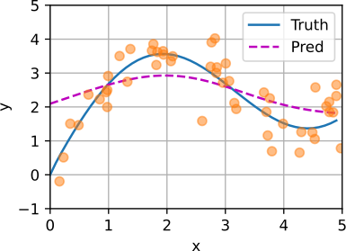
Generate an artificial dataset including 50 training examples and 50 testing examples according to the following nonlinear function with the noise term \epsilon\sim\mathcal{N}(0,0.5) \begin{equation} y=2\sin(x)+x^{0.8}+\epsilon \end{equation}
Find the kernel regression

Nadaraya-Watson Parametric Model

Kernel regression enjoys the consistency benefit: given enough data this model converges to the optimal solution.
Nonetheless, we can easily integrate learnable parameters.
In the following the distance between the query \boldsymbol{x} and the key \boldsymbol{x}_{i} is multiplied a learnable parameter {\color{red}w}:

\begin{equation} \begin{split}\begin{aligned}\hat{y} & =\sum_{i=1}^{N}\frac{\exp\left[-\frac{1}{2}\left(\left\Vert \boldsymbol{x}-\boldsymbol{x}_{i}\right\Vert {\color{red}w}\right)^{2}\right]}{\sum_{j=1}^{N}\exp\left[-\frac{1}{2}\left(\left\Vert \boldsymbol{x}-\boldsymbol{x}_{j}\right\Vert {\color{red}w}\right)^{2}\right]}y_{i}\end{aligned} \end{split} \end{equation}

Example 2

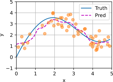
Generate an artificial dataset including 50 training examples and 50 testing examples according to the following nonlinear function with the noise term \epsilon\sim\mathcal{N}(0,0.5) \begin{equation} y=2\sin(x)+x^{0.8}+\epsilon \end{equation}

Find the parametric kernel regression

5.4 Clustering

Clustering

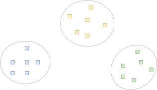
Cluster analysis or clustering is the task of grouping a set of objects in such a way that objects in the same group (called a cluster) are more similar (in some sense) to each other than to those in other groups (clusters).

k-Means

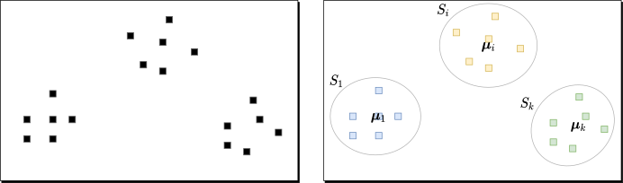
Given a set of observations \mathcal{D}=\{\boldsymbol{x}_{1},\ldots,\boldsymbol{x}_{N}\}, k-means clustering aims to partition the N observations into k (\leq N) sets \boldsymbol{S}=\{S_{1},S_{2},...,S_{k}\} so as to minimize the within-cluster sum of squares

The objective to find \begin{equation} \arg\min_{\boldsymbol{S}}\sum_{i=1}^{k}\sum_{\boldsymbol{x}\in S_{i}}\left\Vert \boldsymbol{x}-\boldsymbol{\mu}_{i}\right\Vert ^{2} \end{equation} where \boldsymbol{\mu}_{i} is the mean of S_{i}

Illustration

Naive k-Means Algorithm

Initialise a set of k means \boldsymbol{m}_{1}^{(0)},…,\boldsymbol{m}_{k}^{(0)}
For t=1,2,3,... do
- Assignment step: Assign each observation to the cluster with the nearest mean: that with the least squared Euclidean distance
\begin{equation} S_{i}^{(t)}=\left\{ \boldsymbol{x}\mid L_{2}(\boldsymbol{x},\boldsymbol{m}_{i}^{(t)})<L_{2}(\boldsymbol{x},\boldsymbol{m}_{j}^{(t)}),\forall j\neq i\right\} \end{equation}
- Update step: Recalculate means (centroids) for observations assigned to each cluster.
\begin{equation} \boldsymbol{m}_{i}^{(t+1)}=\frac{1}{|S_{i}^{(t)}|}\sum_{\boldsymbol{x}\in S_{i}^{(t)}}\boldsymbol{x} \end{equation}

The algorithm has converged when the assignments no longer change

Hierarchical Clustering

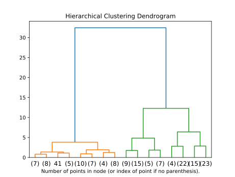
Hierarchical clustering is a method of cluster analysis which seeks to build a hierarchy of clusters.

Linkage Function

A linkage function L is used to calculate the distance (similarity/dissimilarity) between arbitrary subsets of the instance space, given a distance metric d

Single linkage: defines the distance between two clusters as the smallest pairwise distance between elements from each cluster. \begin{equation} L_{single}(A,B)=\min\{d(\boldsymbol{x},\boldsymbol{y})\mid\boldsymbol{x}\in A,\boldsymbol{y}\in B\} \end{equation}
Complete linkage: defines the distance between two clusters as the largest pointwise distance. \begin{equation} L_{complete}(A,B)=\max\{d(\boldsymbol{x},\boldsymbol{y})\mid\boldsymbol{x}\in A,\boldsymbol{y}\in B\} \end{equation}

Agglomerative algorithm

Given a set of observations \mathcal{D}=\{\boldsymbol{x}_{1},\ldots,\boldsymbol{x}_{n}\}

Initialise clusters to singleton data points

Create a leaf node for every singleton cluster

Repeat

find the pair of clusters X, Y with lowest linkage

merge X, Y into Z

create a node for Z (parent node of X, Y)

Until all data points are in one cluster

Return the constructed binary tree

k-d Tree

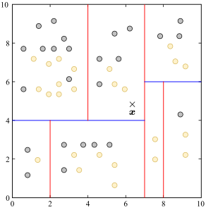
The fundamental problem of k-NN is that distance computation is costly and the total cost unavoidably linear in the number of points compared.
To increase the processing speed, it is possible to partition the data space and reduce this number significantly using k-d tree

A k-d tree (short for k-dimensional tree) is a space-partitioning data structure for organizing points in a k-dimensional space

Algorithm

Construct k-d tree

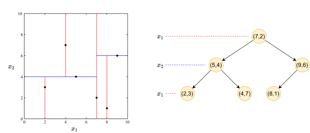
Given and D-dimensional dataset \mathcal{D}=\{\boldsymbol{x}_{1},\boldsymbol{x}_{2},...,\boldsymbol{x}_{N}\}
Cut data with a plane at its median value along that dimension
Recurse this procedure to create a balanced binary tree k-d tree

Nearest neighbor search

Example

Given a dataset \mathcal{D}=\{(x_{1},x_{2})\}=\{(2,3),(5,4),(9,6),(4,7),(8,1),(7,2)\}

Construct k-d tree
Nearest neighbor search