6 STATISTICAL LEARNING
Notation
| symbol | meaning |
|---|---|
| a,b,c,N\dots | scalar number |
| \boldsymbol{w},\boldsymbol{v},\boldsymbol{x},\boldsymbol{y}\dots | column vector |
| \boldsymbol{X},\boldsymbol{Y}\dots | matrix |
| \mathbb{R} | set of real numbers |
| \mathbb{Z} | set of integer numbers |
| \mathbb{N} | set of natural numbers |
| \mathbb{R}^{D} | set of vectors |
| \mathcal{D},\mathcal{X},\mathcal{Y},\dots | set |
| \mathcal{A} | algorithm |
| symbol | meaning |
|---|---|
| X,Y\dots | random variable |
| \boldsymbol{X},\boldsymbol{Y}\dots | multivariate random variable |
| x,y\dots | value |
| \boldsymbol{x},\boldsymbol{y}\dots | vector |
| p,pr,P,Pr | probability |
6.1 Probability And Statistics
Bayes Theorem
\begin{equation} P(h\mid\mathcal{D})=\frac{P(\mathcal{D}\mid h)P(h)}{P(\mathcal{D})} \end{equation}
P(h) = prior probability of hypothesis h
P(\mathcal{D}) = prior probability of observed data \mathcal{D}
P(h\mid\mathcal{D}) = probability of h given \mathcal{D} (called posterior probability)
P(\mathcal{D}\mid h) = probability of \mathcal{D} given h (called likelihood)
Basic Formulas for Probabilities
Given two random variables X and Y, we say that
The quantity p(X,Y) is a joint probability
The quantity p(Y\mid X) is a conditional probability
The quantity p(X) is a marginal probability
Example 1
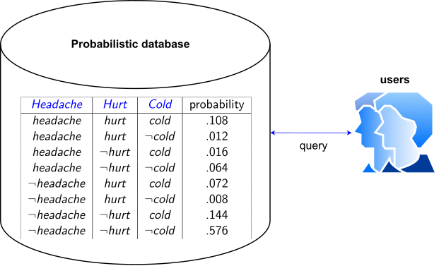
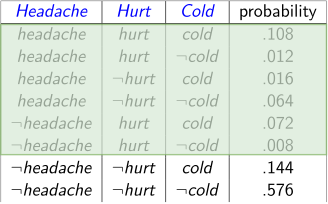
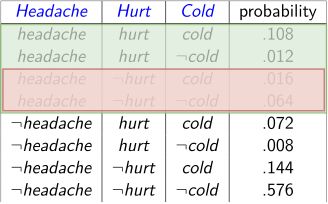
- We have the joint distribution of three random variables P(Headache,Hurt,Cold)
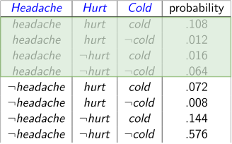
\begin{align*} P(headache) & =0.108+0.012+0.016+0.064\\ & =0.2 \end{align*}
\begin{align*} P(hurt\lor headache) & =0.108+0.012+0.072+0.008+0.016+0.064\\ & =0.28 \end{align*}
\begin{align} P(\lnot hurt\mid headache) & = & \frac{P(\lnot hurt\land headache)}{P(headache)}\\ & = & \frac{0.016+0.064}{0.108+0.012+0.016+0.064}\\ & = & 0.4 \end{align}
Problem Let \boldsymbol{X} be all the variables. We want the posterior joint distribution of the query variables \boldsymbol{Y} given specific values \boldsymbol{e} for the evidence variables \boldsymbol{E}
Proof. Summing solution.
General idea: compute distribution on query variable by fixing evidence variables and summing over hidden variables
Let the hidden variables be \boldsymbol{H}=\boldsymbol{X}-\boldsymbol{Y}-\boldsymbol{E} and denominator can be viewed as a normalization constant \alpha \begin{equation} P(\boldsymbol{Y}\mid\boldsymbol{E}=\boldsymbol{e})=\alpha\:P(\boldsymbol{Y},\boldsymbol{E}=\boldsymbol{e})=\alpha\:\sum_{\boldsymbol{h}}P(\boldsymbol{Y},\boldsymbol{E}=\boldsymbol{e},\boldsymbol{H}=\boldsymbol{h}) \end{equation}
◻
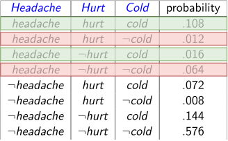
\begin{align} & & P(Hurt\mid headache)\\ & = & \alpha\,P(Hurt,headache)\\ & = & \alpha\,[P(Hurt,headache,cold)+P(Hurt,headache,\lnot cold)]\\ & = & \alpha\,[\left\langle 0.108,0.016\right\rangle +\left\langle 0.012,0.064\right\rangle ]\\ & = & \alpha\,\left\langle 0.12,0.08\right\rangle \\ & = & \left\langle 0.6,0.4\right\rangle \end{align}
6.2 Statistical Learning
Statistical Model
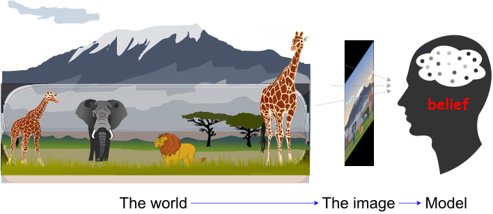
- All models are wrong, but some are useful (statistical model) - George Box
Probabilistic Approach
Learning is an estimation of joint probability density function p(\boldsymbol{x},y) given observed data \mathcal{D}. Inductive bias is expressed as prior assumptions about these joint distributions.
Classification and Regression: conditional density estimation \begin{equation} p(y\mid\boldsymbol{x}) \end{equation}
Unsupervised Learning: density estimation \begin{equation} p(\boldsymbol{x}) \end{equation}
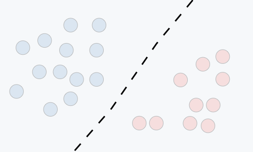
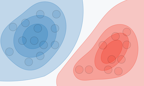
Type of Supervised Model
| Discriminative model | Generative model | |
|---|---|---|
| Goal |
|
|
| What’s learned |
|
|
 |
 |
Bayesian Learning
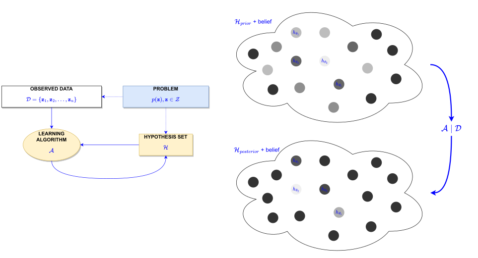
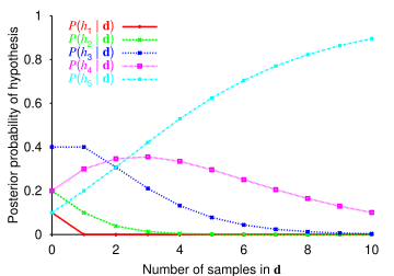
Bayesian learning is a process that updates of a probability distribution (belief) over the hypothesis space \mathcal{H}=\{h_{1},h_{2},...\} given samples \mathcal{D}.
Prior probability of each hypothesis h_{i} \begin{equation} P(h_{i}) \end{equation}
Given the data \mathcal{D}, each hypothesis has a posterior probability (update) \begin{equation} P(h_{i}\mid\mathcal{D})=\alpha P(\mathcal{D}\mid h_{i})P(h_{i}) \end{equation}
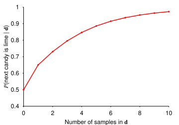
Predictions use an average over the hypotheses \begin{equation} P(d)=\sum_{i}P(d\mid h_{i})P(h_{i}) \end{equation}
Components of Learning
Evolution of Posterior Probabilities
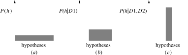
- Changes of a probability distribution P(h) after observing the data D_{1} and D_{2}
Example 1
Does patient have COVID or not?
“A patient takes a lab test and the result comes back positive. The test returns a correct positive result in only 98\% of the cases in which the disease is actually present, and a correct negative result in only 97\% of the cases in which the disease is not present. Furthermore, .008 of the entire population have this COVID.”
Proof. Solution.
| P(COVID) | = | ______ | P(\neg COVID) | = | ______ |
| P(\oplus\mid COVID) | = | ______ | P(\ominus\mid COVID) | = | ______ |
| P(\oplus\mid\neg COVID) | = | ______ | P(\ominus\mid\neg COVID) | = | ______ |
◻
Example 2
Suppose there are five kinds of bags of candies:
10% are h_{1}: 100% cherry candies
20% are h_{2}: 75% cherry candies + 25% lime candies
40% are h_{3}: 50% cherry candies + 50% lime candies
20% are h_{4}: 25% cherry candies + 75% lime candies
10% are h_{5}: 100% lime candies
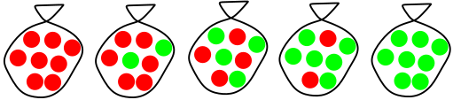
Experiment
Select one bag
Candies drawn from the bag:

Question
What kind of bag is it?
What flavour will the next candy be?
What kind of bag is it?
Posterior probability of hypotheses
What flavour will the next candy be?
Prediction probability
Exercise
Suppose we have a box of dice that contains a 4-sided die, a 6-sided die, an 8-sided die, a 12-sided die, and a 20-sided die
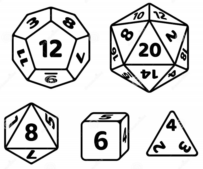
Experiment
We select one die
We roll the die a few more times and get \mathcal{D}=\{6,8,7,7,5,4\}
Question
- What die is selected?
6.3 Fitting Models
Learning Strategy
Fitting probability models to data \mathcal{D}=\left\{ \boldsymbol{x}_{1},...\boldsymbol{x}_{n}\right\} is referred to as learning because we learn about the parameters \theta of the model
Updating or summing over the hypothesis space is often intractable (e.g., 18,446,744,073,709,551,616 Boolean functions of 6 attributes)
Alternative strategies:
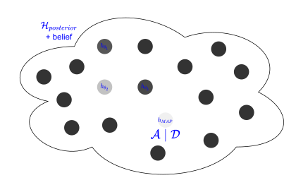
Maximum a posteriori (MAP) learning
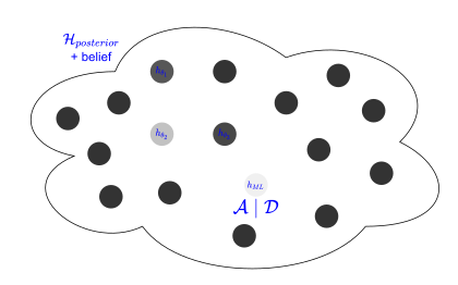
Maximum likelihood (ML) learning
Maximum a posteriori
Given data \mathcal{D}
choose hypothesis h (called h_{MAP}) maximizing P(h\mid\mathcal{D})
i.e., maximize P(\mathcal{D}\mid h)P(h) or \log P(\mathcal{D}\mid h)+\log P(h)
Maximum likelihood
For large data sets, prior becomes weak or irrelevant, maximum likelihood learning
Given data \mathcal{D}, choose hypothesis h (called h_{ML}) maximizing P(\mathcal{D}\mid h) or \log P(\mathcal{D}\mid h)
One categorical variable
Example 1
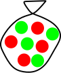
A bag containing two kinds of candies, lime and cherry, has a fraction {\color{red}\theta} of cherry candies?
Experiment
Candies drawn from the bag:

Question
- What the value of {\color{red}\theta} is?
Proof. ML learning solution.
- The model (Bayes net) has one variable flavor with one parameter {\color{red}\theta}

Any {\color{red}\theta}\in[0,1] is possible: continuum of hypotheses h_{{\color{red}\theta}}
{\color{red}\theta} is a parameter for this simple (binomial) family of models
Suppose we unwrap N candies, c cherries and \ell=N-c limes. These are i.i.d. (independent, identically distributed) observations, so p(\mathcal{D}\mid h_{{\color{red}\theta}})=\prod_{j=1}^{N}p(d_{j}\mid h_{{\color{red}\theta}})={\color{red}\theta}^{c}\cdot(1-{\color{red}\theta})^{\ell}
Maximize this w.r.t. {\color{red}\theta}—which is easier for the log-likelihood: \begin{align} L(\mathcal{D}\mid h_{{\color{red}\theta}}) & = & \log p(\mathcal{D}\mid h_{{\color{red}\theta}})\nonumber \\ & = & \sum_{j=1}^{N}\log p(d_{j}\mid h_{{\color{red}\theta}})\nonumber \\ & = & c\log{\color{red}\theta}+\ell\log(1-{\color{red}\theta})\nonumber \\ \frac{dL(\mathcal{D}\mid h_{{\color{red}\theta}})}{d{\color{red}\theta}} & = & \frac{c}{{\color{red}\theta}}-\frac{\ell}{1-{\color{red}\theta}}=0\nonumber \\ \implies{\color{red}\theta_{ML}} & = & \frac{c}{c+\ell}=\frac{c}{N} \end{align}
◻
- ML seems sensible, but causes problems with 0 counts!
Proof. MAP learning solution.
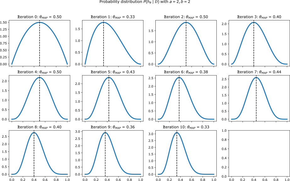
Prior for h_{{\color{red}\theta}} p(h_{{\color{red}\theta}})=Beta(a,b)\text{ where }a,b>0,
Posteriori for h_{{\color{red}\theta}} given \mathcal{D} \begin{align*} p(h_{{\color{red}\theta}}\mid\mathcal{D}) & \propto p(\mathcal{D}\mid h_{{\color{red}\theta}})p(h_{{\color{red}\theta}})\\ & =Beta(a+c,b+\ell) \end{align*}
MAP estimate \begin{equation} {\color{red}\theta_{MAP}}=\frac{c+a-1}{c+\ell+a+b-2} \end{equation}
◻
Two categorical variables
Example 2
A bag has a fraction {\color{red}\theta} of cherry candies, red/green wrapper depends probabilistically {\color{red}\theta_{1}},{\color{red}\theta_{2}} on flavor?
Experiment
Candies drawn from some bag \mathcal{D}

Question
- What the values of {\color{red}\theta},{\color{red}\theta_{1}},{\color{red}\theta_{2}} are?
Proof. ML learning solution.
- The model (Bayes net) has two variables flavor and wrapper with three parameters {\color{red}\theta},{\color{red}\theta_{1}},{\color{red}\theta_{2}}
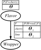
Likelihood for, e.g., cherry candy in green wrapper: \begin{array}{l} p(F=cherry,W=green\mid h_{{\color{red}\theta},{\color{red}\theta_{1}},{\color{red}\theta_{2}}})\\ =p(F=cherry\mid h_{{\color{red}\theta},{\color{red}\theta_{1}},{\color{red}\theta_{2}}})p(W=green\mid F=cherry;h_{{\color{red}\theta},{\color{red}\theta_{1}},{\color{red}\theta_{2}}})\\ ={\color{red}\theta}\cdot(1-{\color{red}\theta_{1}}) \end{array}
N candies, r_{c} red-wrapped cherry candies, etc.: \begin{align} p(\mathcal{D}\mid h_{{\color{red}\theta},{\color{red}\theta_{1}},{\color{red}\theta_{2}}}) & = & {\color{red}\theta}^{c}(1-{\color{red}\theta})^{\ell}\cdot{\color{red}\theta}_{{\color{red}1}}^{r_{c}}(1-{\color{red}\theta_{1}})^{g_{c}}\cdot{\color{red}\theta}_{{\color{red}2}}^{r_{\ell}}(1-{\color{red}\theta_{2}})^{g_{\ell}} \end{align}
\begin{align} L & = & [c\log{\color{red}\theta}+\ell\log(1-{\color{red}\theta})]\\ & & +[r_{c}\log{\color{red}\theta}_{{\color{red}1}}+g_{c}\log(1-{\color{red}\theta_{1}})]\\ & & +[r_{\ell}\log{\color{red}\theta_{2}}+g_{\ell}\log(1-{\color{red}\theta_{2}})] \end{align}
Derivatives of L contain only the relevant parameter: \begin{array}{rclcl} {\displaystyle \frac{\partial L}{\partial{\color{red}\theta}}} & = & {\displaystyle \frac{c}{{\color{red}\theta}}-{\displaystyle \frac{\ell}{1-{\color{red}\theta}}=0}} & \implies & {\color{red}\theta}={\displaystyle \frac{c}{c+\ell}}\end{array}
\begin{array}{rclcl} {\displaystyle \frac{\partial L}{\partial{\color{red}\theta_{1}}}} & = & {\displaystyle \frac{r_{c}}{{\color{red}\theta_{1}}}-{\displaystyle \frac{g_{c}}{1-{\color{red}\theta_{1}}}=0}} & \implies & {\color{red}\theta_{1}}={\displaystyle \frac{r_{c}}{r_{c}+g_{c}}}\end{array}
\begin{array}{rclcl} {\displaystyle \frac{\partial L}{\partial{\color{red}\theta_{2}}}} & = & {\displaystyle \frac{r_{\ell}}{{\color{red}\theta_{2}}}-{\displaystyle \frac{g_{\ell}}{1-{\color{red}\theta_{2}}}=0}} & \implies & {\color{red}\theta_{2}}={\displaystyle \frac{r_{\ell}}{r_{\ell}+g_{\ell}}}\end{array}
With complete data, parameters can be learned separately
◻
One continuous variable
Example 3
Suppose that the distribution of male height is a normal distribution \mathcal{N}({\color{red}\mu},{\color{red}\sigma}^{2}). Given the following data \mathcal{D}
# height (m) # height (m) 1 1.72 6 1.63 2 1.65 7 1.74 3 1.60 8 1.82 4 1.73 9 1.75 5 1.80 10 1.64 Question: what are the values of {\color{red}\mu},{\color{red}\sigma}?
Proof. ML learning solution.
The model has one variable x (height) with two parameters {\color{red}\mu},{\color{red}\sigma}^{2} \begin{equation} p(x\mid{\color{red}\mu},{\color{red}\sigma}^{2})=\mathcal{N}(x\mid{\color{red}\mu},{\color{red}\sigma}^{2})=\frac{1}{\sqrt{2\pi{\color{red}\sigma}^{2}}}\exp\left[-\frac{(x-{\color{red}\mu})^{2}}{2{\color{red}\sigma}^{2}}\right] \end{equation}
The likelihood of model with the parameters \{{\color{red}\mu},{\color{red}\sigma}^{2}\} for observed i.d.d. data \mathcal{D}=\{x_{1},...,x_{n}\} is \begin{align} p(\mathcal{D}\mid{\color{red}\mu},{\color{red}\sigma}^{2}) & = & \prod_{i=1}^{n}\mathcal{N}(x_{i}\mid{\color{red}\mu},{\color{red}\sigma}^{2})\nonumber \\ & = & \frac{1}{(2\pi{\color{red}\sigma}^{2})^{n/2}}\exp\left[-\frac{1}{2}\sum_{i=1}^{n}\frac{(x_{i}-{\color{red}\mu})^{2}}{{\color{red}\sigma}^{2}}\right] \end{align}
The maximum likelihood solution {\color{red}\mu_{ML}}, {\color{red}\sigma}_{{\color{red}ML}}^{2} \begin{equation} {\color{red}\mu_{ML}},{\color{red}\sigma}_{{\color{red}ML}}^{2}=\text{argmax}_{{\color{red}\mu},{\color{red}\sigma}^{2}}[p(\mathcal{D}\mid{\color{red}\mu},{\color{red}\sigma}^{2})] \end{equation}
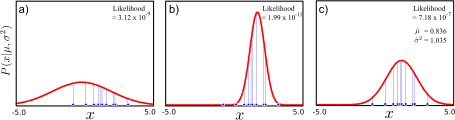
Since the logarithm is a monotonic function, the position of the maximum in the transformed function L=\log p(\mathcal{D}\mid{\color{red}\mu},{\color{red}\sigma}^{2}) remains the same as p(\mathcal{D}\mid{\color{red}\mu},{\color{red}\sigma}^{2})
The maximum log-likelihood solution \begin{align} {\color{red}\mu_{ML}},{\color{red}\sigma}_{{\color{red}ML}}^{2} & = & \text{argmax}_{{\color{red}\mu},{\color{red}\sigma}^{2}}[\log p(\mathcal{D}\mid{\color{red}\mu},{\color{red}\sigma}^{2})]\nonumber \\ & = & \text{argmax}_{{\color{red}\mu},{\color{red}\sigma}^{2}}\left[-\frac{1}{2}n\log[2\pi]-\frac{1}{2}\log{\color{red}\sigma}^{2}-\frac{1}{2}\sum_{i=1}^{n}\frac{(x_{i}-{\color{red}\mu})^{2}}{{\color{red}\sigma}^{2}}\right]. \end{align}
- To maximize, we differentiate this log-likelihood L with respect to \mu and equate the result to zero \begin{align} \frac{\partial L}{\partial{\color{red}\mu}} & = & \sum_{i=1}^{n}\frac{(x_{i}-{\color{red}\mu})}{{\color{red}\sigma}^{2}}\nonumber \\ & = & \frac{\sum_{i=1}^{n}x_{i}}{{\color{red}\sigma}^{2}}-\frac{n{\color{red}\mu}}{{\color{red}\sigma}^{2}}=0\nonumber \\ {\color{red}\mu_{ML}} & = & \frac{1}{n}\sum_{i=1}^{n}x_{i} \end{align}
- By a similar process, the expression for the variance can be shown to be
\begin{equation} {\color{red}\sigma}_{{\color{red}ML}}^{2}=\frac{1}{n}\sum_{i=1}^{n}(x_{i}-{\color{red}\mu_{ML}})^{2}. \end{equation} ◻
Joint Probability Distributions
Joint Probability Distributions
The joint probability distribution is central to probabilistic inference, because once we know the joint distribution we can answer every possible probabilistic question that can be asked about these variables.
Gender HoursWorked Wealth probability female <40.5 poor 0.2531 female <40.5 rich 0.0246 female \geq40.5 poor 0.0422 female \geq40.5 rich 0.0116 male <40.5 poor 0.3313 male <40.5 rich 0.0972 male \geq40.5 poor 0.1341 male \geq40.5 rich 0.1059
Discussion
- How can we learn joint distributions from observed training data \mathcal{D}?
6.4 Linear Regression Revisited
Linear Regression
Linear regression without prior belief
Linear regression with prior belief
Linear Regression Revisited
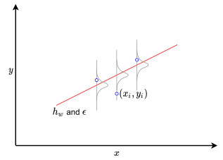
Unknown function f is modeled by the hypothesis h_{{\color{red}\boldsymbol{w}}} \begin{equation} y=h_{\boldsymbol{{\color{red}w}}}(x)=\boldsymbol{{\color{red}w}}^{\intercal}\boldsymbol{x}+\epsilon \end{equation} where y is noisy target value, \epsilon is random variable (noise) drawn independently according to a Gaussian distribution with mean equal to 0 and variance equal to {\color{red}\sigma} (\mathcal{N}(0,{\color{red}\sigma}^{2}))
Probability language \begin{equation} p(y\mid\boldsymbol{x},{\color{red}\boldsymbol{w}})=\mathcal{N}(y\mid\boldsymbol{{\color{red}w}}^{\intercal}\boldsymbol{x},{\color{red}\sigma}^{2}) \end{equation}
Given data \mathcal{D}=\{\boldsymbol{x}_{i},y_{i}\}_{i=1}^{N}, the likelihood of \mathcal{D} given h_{{\color{red}\boldsymbol{w}}} and noise
\begin{equation} \begin{array}{rcl} p(\mathcal{D}\mid h_{\boldsymbol{{\color{red}w}}},\epsilon) & = & \prod_{i=1}^{N}p(y_{i}\mid\boldsymbol{x}_{i},\boldsymbol{{\color{red}w}})\\ & = & \prod_{i=1}^{N}\mathcal{N}(y_{i}\mid\boldsymbol{{\color{red}w}}^{\intercal}\boldsymbol{x}_i,{\color{red}\sigma}^{2}) \end{array} \end{equation}
ML Learning
Choose hypothesis h maximizing the likelihood \begin{equation} \begin{array}{cl} & \arg\max_{\boldsymbol{{\color{red}w}},{\color{red}\sigma}}p(\mathcal{D}\mid h_{\boldsymbol{{\color{red}w}}},e)\\ \Leftrightarrow & \arg\max_{\boldsymbol{{\color{red}w}},{\color{red}\sigma}}\prod_{i=1}^{N}\mathcal{N}(y_{i}\mid\boldsymbol{{\color{red}w}}^{\intercal}\boldsymbol{x}_{i},{\color{red}\sigma}^{2})\\ \Leftrightarrow & \arg\max_{\boldsymbol{{\color{red}w}},{\color{red}\sigma}}\log\left(\prod_{i=1}^{N}\mathcal{N}(y_{i}\mid\boldsymbol{{\color{red}w}}^{\intercal}\boldsymbol{x}_{i},{\color{red}\sigma}^{2})\right)\\ \Leftrightarrow & \arg\min_{\boldsymbol{{\color{red}w}},{\color{red}\sigma}}\dfrac{1}{2{\color{red}\sigma}^{2}}MSE+\dfrac{N}{2}\log({\color{red}\sigma}^{2})+\dfrac{N}{2}\log(2\pi) \end{array} \end{equation}
Solving (20), we have
\boldsymbol{{\color{red}w}}_{ML}=(\boldsymbol{X}^{\intercal}\boldsymbol{X})^{-1}\boldsymbol{X}^{\intercal}\boldsymbol{y}
{\color{red}\sigma}_{ML}^{2}=\frac{1}{N}\sum_{i=1}^{N}({\color{red}\boldsymbol{w}}_{ML}^{\intercal}\boldsymbol{x}_{i}-y_{i})^{2}
Example
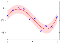
The red curve denotes the regression curve and the red region corresponds to \pm{\color{red} \sigma} standard deviation
Bayesian Learning
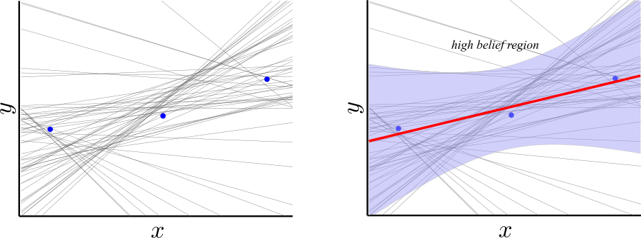
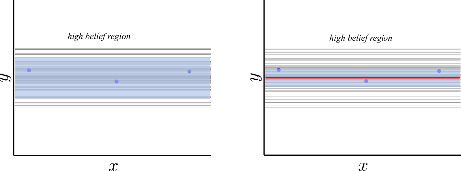
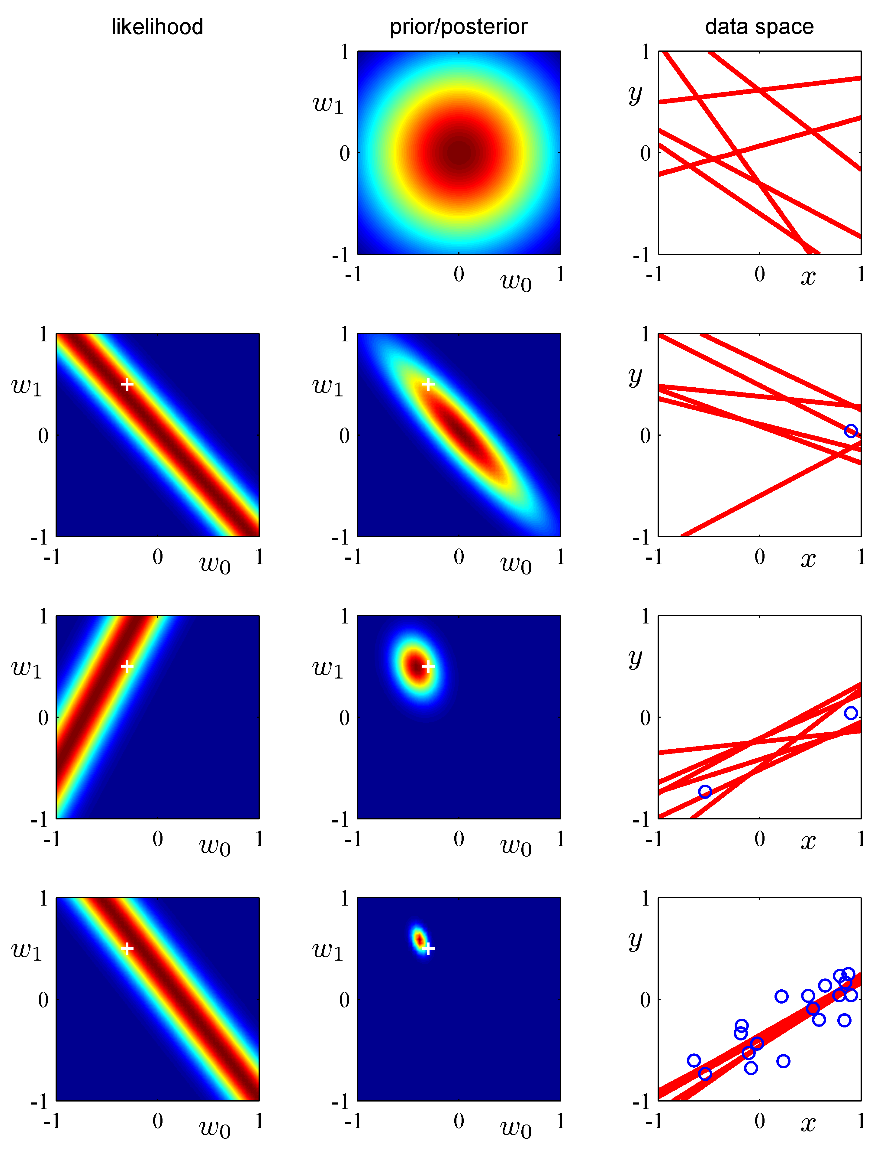
The figure shows the update process of Bayesian learning where \boldsymbol{{\color{red}w}} are introduced as hypothesis parameters
6.5 Naive Bayes
When to use
Along with decision trees, neural networks, nearest neighbour, one of the most practical learning methods.
Moderate or large training set available
Attributes that describe instances are conditionally independent given classification
Successful applications
Diagnosis
Classifying text documents
Naive Bayes assumption
Assume target function for classification problem f:\mathcal{X}\rightarrow\mathcal{Y} where each instance \boldsymbol{x} described by attributes (x_{1},x_{2}\ldots x_{D}) and y is a corresponding class.
Naive Bayes assumption \begin{equation} P(x_{1},x_{2}\ldots x_{D}\mid y)=\prod_{i=1}^{D}P(x_{i}\mid y) \end{equation}
Naive Bayes classifiers
- Naive Bayes classifier
\begin{equation} y_{NB}=\arg\max_{y}\hat{P}(y)\prod_{i=1}^{D}\hat{P}(x_{i}\mid y) \end{equation}
The form of the class-conditional density depends on the type of each feature.
In the case of real-valued features, we can use the Gaussian distribution: p(\boldsymbol{x}\mid y=c)\sim\prod_{j=1}^{D}\mathcal{N}(x_{j}\mid{\color{red}\mu_{jc}},{\color{red}\sigma_{jc}^{2}}) where {\color{red}\mu}_{{\color{red}jc}} is the mean of feature j in objects of class c, and {\color{red}\sigma}_{{\color{red}jc}}^{{\color{red}2}} is its variance.
In the case of binary features, x_{j}\in\{0,1\}, we can use the Bernoulli distribution: p(\boldsymbol{x}\mid y=c)\sim\prod_{j=1}^{D}\text{Ber}(x_{j}\mid{\color{red}\mu_{jc}}) where {\color{red}\mu}_{{\color{red}jc}} is the probability that feature j occurs in class c.
In the case of categorical features, x_{j}\in\{v_{j_{1}},v_{j_{2}},\cdots,v_{j_{K}}\}, we can use the multinoulli distribution: p(\boldsymbol{x}\mid y=c)\sim\prod_{j=1}^{D}\text{Cat}(x_{j}\mid{\color{red}\boldsymbol{\mu}}_{{\color{red}jc}}) where {\color{red}\boldsymbol{\mu}}_{{\color{red}jc}} is a histogram over the K possible values for x_{j} in class c.
Naive Bayes Algorithm
LearnNaiveBayes(\mathcal{D})
for each target value (class) y_{j}
\hat{P}(y_{j}) \leftarrow estimate P(y_{j}) given data \mathcal{D}
for each attribute x_{i}
\hat{P}(x_{i}\mid y_{j}) \gets estimate P(x_{i}\mid y_{j}) given data \mathcal{D}
ClassifyNewInstance(x)
y=\arg\max_{y}\hat{P}(y)\prod_{i=1}^{D}\hat{P}(x_{i}\mid y)
return y
Maximum likelihood learning for \hat{P}(y=c) and \hat{P}(x_{i}=a\mid y=c) \begin{equation} \hat{P}(y=c)\gets\frac{n_{c}}{n} \end{equation}
\begin{equation} \hat{P}(x_{i}=a\mid y=c)\leftarrow\frac{n_{a}}{n_{c}} \end{equation} where
n is number of training examples
n_{c} is number of training examples for which y=c
n_{a} is number of examples for which y=c and x_{i}=a
Example 1
Consider PlayTennis again
Day Outlook Temperature Humidity Wind PlayTennis? D1 sunny hot high weak no D2 sunny hot high strong no D3 overcast hot high weak yes D4 rain mild high weak yes D5 rain cool normal weak yes D6 rain cool normal strong no D7 overcast cool normal strong yes D8 sunny mild high weak no D9 sunny cool normal weak yes D10 rain mild normal weak yes D11 sunny mild normal strong yes D12 overcast mild high strong yes D13 overcast hot normal weak yes D14 rain mild high strong no Naive Bayes model
\hat{P}(PlayTennis)
|
|||||||||||||||||||||||||||||||||||||||
\hat{P}(Outlook\mid PlayTennis)
|
\hat{P}(Temperature\mid PlayTennis)
|
||||||||||||||||||||||||||||||||||||||
\hat{P}(Humidity\mid PlayTennis)
|
\hat{P}(Wind\mid PlayTennis)
|
||||||||||||||||||||||||||||||||||||||
Get new instance
\boldsymbol{x}=(Outlk=sun,Temp=cool,Humid=high,Wind=strong)
Compute
\begin{cases} \hat{P}(yes)\times\hat{P}(sun\mid yes)\times\hat{P}(cool\mid yes)\times\hat{P}(high\mid yes)\times\hat{P}(strong\mid yes) & =.005\\ \hat{P}(no)\times\hat{P}(sun\mid no)\times\hat{P}(cool\mid no)\times\hat{P}(high\mid no)\times\hat{P}(strong\mid no) & =.021 \end{cases}
Make decison
y=no
Example 2
Find Naive Bayes classifier given the following training dataset
# Vị Màu Vỏ Độc tính 1 ngọt đỏ nhẵn không 2 cay đỏ nhẵn có 3 chua vàng có gai không 4 cay vàng có gai có 5 ngọt tím có gai không 6 chua vàng nhẵn không 7 ngọt tím nhẵn không 8 cay tím có gai có 9 cay tím có gai không 10 cay tím có gai có 11 cay vàng có gai có
Avoiding the zero-probability problem
Conditional independence assumption is often violated but it works surprisingly well anyway
Suppose that none of the training instances with target value y have attribute value x_{i}=v? then \hat{P}(x_{i}=v\mid y)=0, and \hat{P}(y)\dots\hat{P}(x_{i}=v\mid y)\dots=0 (not good in probability language)
Typical solution is Bayesian estimate for \hat{P}(y=c) and \hat{P}(x_{i}=a\mid y=c) \begin{equation} \hat{P}(y=c)\gets\frac{n_{c}+1}{n+C} \end{equation}
\begin{equation} \hat{P}(x_{i}=a\mid y=c)\leftarrow\frac{n_{a}+1}{n_{c}+r} \end{equation} where
n is number of training examples
n_{c} is number of training examples for which y=c
C is the number of classes
n_{a} is number of examples for which y=c and x_{i}=a
r is the number of values of attribute x_{i}
Example 3
Find Naive Bayes classifier given the following training dataset
# Height (m) Hair Gender 1 1.72 brown male 2 1.65 black female 3 1.60 black female 4 1.73 black female 5 1.80 brown male 6 1.63 black male 7 1.74 black female 8 1.82 brown male 9 1.75 black male 10 1.64 brown female
6.6 Statistical Language Model
Language Models
A language model is a function p_{\text{\text{lm}}} that takes an English (or any language) sentence and returns the probability that it was produced by an English speaker

Answer the question: How likely is a string of English (or any language) words good English?
Help with reordering p_{\text{\text{lm}}}(\text{the house is small})>p_{\text{\text{lm}}}(\text{small the is house})
Help with word choice p_{\text{\text{lm}}}(\text{I am going home})>p_{\text{\text{lm}}}(\text{I am going house})
Given a string of English words W=w_{1},w_{2},w_{3},...,w_{n}. Question: what is p(W)?
Decomposing p(W) using the chain rule: \begin{equation} p(w_{1},w_{2},w_{3},...,w_{n})=p(w_{1})\;p(w_{2}|w_{1})\;p(w_{3}|w_{1},w_{2})...p(w_{n}|w_{1},w_{2},...w_{n-1}) \end{equation}
The language model probability p(w_{1},w_{2},w_{3},...,w_{n}) is a product of word history probabilities given a history of preceding words.
Markov Assumption
Markov assumption states that only a limited number of previous words affect the probability of the next word.
- limited memory: only last k words are included in history (older words less relevant) \rightarrow kth order Markov model
N-Gram Language Models
Unigram (1-gram) model \begin{equation} p(w_{1},w_{2},w_{3},...,w_{n})=p(w_{1})\;p(w_{2})\;p(w_{3})...p(w_{n}) \end{equation}
Bigram (2-gram) model \begin{equation} p(w_{1},w_{2},w_{3},...,w_{n})={\color{lightgray}p(w_{1}}\mathclose{\color{lightgray})}\;p(w_{2}|w_{1})\;p(w_{3}|w_{2})...p(w_{n}|w_{n-1}) \end{equation}
Trigram (3-gram) model \begin{equation} p(w_{1},w_{2},w_{3},...,w_{n})={\color{lightgray}p(w_{1})\;p(w_{2}|w_{1}}\mathclose{\color{lightgray})}\;p(w_{3}|w_{1},w_{2})...p(w_{n}|w_{n-2},w_{n-1}) \end{equation}
Estimating N-Gram Probabilities
Maximum likelihood estimation for 1-gram \begin{equation} p_{\text{\text{lm}}}(w_{1})=\frac{\text{count}(w_{1})}{\text{the total number of words}} \end{equation}
Maximum likelihood estimation for 2-gram \begin{equation} p_{\text{\text{lm}}}(w_{2}|w_{1})=\frac{\text{count}(w_{1},w_{2})}{\text{count}(w_{1})} \end{equation}
Maximum likelihood estimation for 3-gram \begin{equation} p_{\text{\text{lm}}}(w_{3}|w_{1},w_{2})=\frac{\text{count}(w_{1},w_{2},w_{3})}{\text{count}(w_{1},w_{2})} \end{equation}
Example 1
Given a corpus
<s> I am Sam </s>
<s> Sam I am </s>
<s> I do not like ham </s>
Some of the bigram probabilities from this corpus p_{\text{\text{lm}}}(w_{2}|w_{1})=\frac{\text{count}(w_{1},w_{2})}{\text{count}(w_{1})}
p_{\text{\text{lm}}}(\text{\texttt{I}}|\text{\texttt{<s>}})=\frac{2}{3}=0.67
p_{\text{\text{lm}}}(\text{\texttt{Sam}}|\text{\texttt{<s>}})=\frac{1}{3}=0.33
p_{\text{\text{lm}}}(\text{\texttt{am}}|\text{\texttt{I}})=\frac{2}{3}=0.67
p_{\text{\text{lm}}}(\text{\texttt{do}}|\text{\texttt{I}})=\frac{1}{3}=0.33
p_{\text{\text{lm}}}(\text{\texttt{Sam}}|\text{\texttt{am}})=\frac{1}{2}=0.5
p_{\text{\text{lm}}}(\text{\texttt{</s>}}|\text{\texttt{Sam}})=\frac{1}{2}=0.5
Exercise 1
Given a corpus
<s> Tôi là nam </s>
<s> Bạn tôi là nữ </s>
<s> Tôi thích trà </s>
Compute all the bigram probabilities from this corpus
Example 2
- Bigram probabilities for eight words (out of V=1446) in the Berkeley Restaurant Project corpus of 9332 sentences. Zero probabilities are in gray
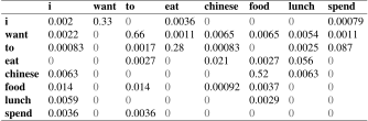
And a few other useful probabilities \begin{array}{ll} p_{\text{\text{lm}}}(\text{\texttt{i}}|\text{\texttt{<s>}})=0.25 & p_{\text{\text{lm}}}(\text{\texttt{english}}|\text{\texttt{want}})=0.0011\\ p_{\text{\text{lm}}}(\text{\texttt{food}}|\text{\texttt{english}})=0.5 & p_{\text{\text{lm}}}(\text{\texttt{</s>}}|\text{\texttt{food}})=0.68 \end{array}
Compute the probability of sentences like
I want English foodorI want Chinese foodThe probability of sentence
I want English food\to<s> i want english food </s># p(w_{2}|w_{1}) value 1 p_{\text{\text{lm}}}(\text{\texttt{i}}|\text{\texttt{<s>}}) 0.25 2 p_{\text{\text{lm}}}(\text{\texttt{want}}|\text{\texttt{i}}) 0.33 3 p_{\text{\text{lm}}}(\text{\texttt{english}}|\text{\texttt{want}}) 0.0011 4 p_{\text{\text{lm}}}(\text{\texttt{food}}|\text{\texttt{english}}) 0.5 5 p_{\text{\text{lm}}}(\text{\texttt{</s>}}|\text{\texttt{food}}) 0.68 total 0.000031
Practical Issues
We do everything in log space
Avoid underflow
Adding is faster than multiplying
\begin{equation} \log(p_{1}\times p_{2}\times...\times p_{n})=\log(p_{1})+\log(p_{2})+...+\log(p_{n}) \end{equation}
| # | (w_{2}|w_{1}) | p_{\text{\text{lm}}}(w_{2}|w_{1}) | \log_{2}p_{\text{\text{lm}}}(w_{2}|w_{1}) |
|---|---|---|---|
| 1 | (\text{\texttt{i}}|\text{\texttt{<s>}}) | 0.25 | -2.0 |
| 2 | (\text{\texttt{want}}|\text{\texttt{i}}) | 0.33 | -1.6 |
| 3 | (\text{\texttt{english}}|\text{\texttt{want}}) | 0.0011 | -9.8 |
| 4 | (\text{\texttt{food}}|\text{\texttt{english}}) | 0.5 | -1.0 |
| 5 | (\text{\texttt{</s>}}|\text{\texttt{food}}) | 0.68 | -0.6 |
| total | 0.000031 | -15.0 |
Evaluation and Perplexity
A good model assigns a string of words W=w_{1},w_{2},w_{3},...,w_{n} a high probability
There are various ways to measure this \begin{equation} \begin{array}{ll} L=p(w_{1},w_{2},w_{3},...,w_{n}) & \text{(likelihood)}\\ \\H=-\dfrac{1}{n}\log_{2}L & \text{(per-word cross-entropy)}\\ \\PP=2^{H} & \text{(perplexity)} \end{array} \end{equation}
Lower perplexity = better model
Text Generation
Three sentences randomly generated from three n-gram models computed from 40 million words of the Wall Street Journal, lower-casing all characters and treating punctuation as words.

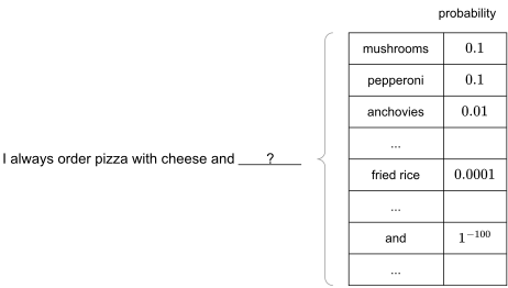
The Shannon Game: How well can we predict the next word?
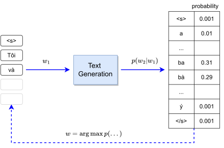
Text generation model
Shortcomings of n-gram models
But there are many more unseen n-grams than seen n-grams
Example, Europarl 2-grams:
86,700 distinct words
86,700^{2}=7,516,890,000 possible 2-grams
but only about 30,000,000 words (and 2-grams) in corpus
Example, Vietnamese 3-grams:
6,814 distinct syllables
6,814^{3}=316,378,081,144 possible 3-grams
but only about 1,500,000 3-grams in corpus
Long-range dependencies
- To capture a dependency between the next word and the word 10 positions in the past, we need to see a relevant 11-gram in the text
Lack of generalization across contexts
- Having observed
black carandblue cardoes not influence our estimates of the eventred carif we haven’t see it before
6.7 Bayesian Networks
Introduction
Bayesian networks
A Bayesian network, or causal probabilistic network, is a directed acyclic graph (DAG) for conditional independence assertions and hence for compact specification of full joint distributions
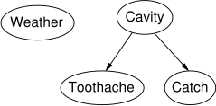
Syntax
Nodes represent variables
Links represent dependency relations between variables and quantified by conditional distributions
A conditional distribution for each node given its parents: P(X_{i}\mid parents(X_{i}))
In the simplest case, conditional distribution represented as a conditional probability table (CPT) giving the distribution over X_{i} for each combination of parent values
Example
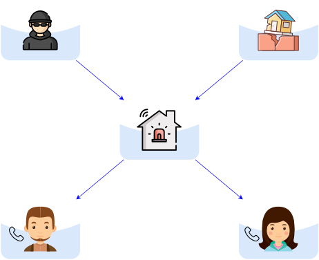
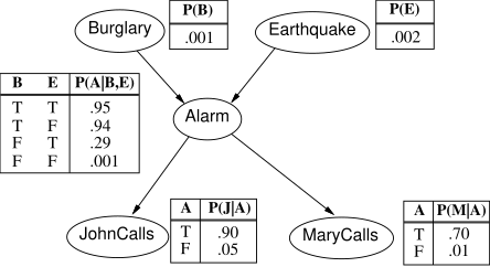
I’m at work, neighbor John calls to say my alarm is ringing, but neighbor Mary doesn’t call. Sometimes it’s set off by minor earthquakes. Is there a burglar?
Variables: \boldsymbol{B}urglar, \boldsymbol{E}arthquake, \boldsymbol{A}larm, \boldsymbol{J}ohnCalls, \boldsymbol{M}aryCalls
Network topology reflects “causal” knowledge:
A burglar can set the alarm off
An earthquake can set the alarm off
The alarm can cause Mary to call
The alarm can cause John to call
Queries
P(Query\mid Evidence)=?
Diagnostic (from effects to causes)
P(B\mid J) \to “If John calls, how likely is the house burglarized?”
Causal (from causes to effects):
P(J\mid E) \to “If earthquake happens, how likely will John make a call?”
Intercausal (between causes of a common effect):
P(B\mid A,E) \to “If earthquake happens and alarm is on, how likely is the house burglarized??”
Mixed:
P(A\mid J,E) \to “...”
P(B\mid J,E) \to “...”
Representation
Graphical Model
Type of Variables
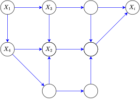
Variables \{X_{i}\}
random or deterministic
observed or hidden
continuous or discrete (boolean, category)
CPT Representation
A CPT for Boolean X_{i} with k Boolean parents has 2^{k} rows for the combinations of parent values
Each row requires one number p for X_{i}=true (the number for X_{i}=false is just 1-p)
If each variable has no more than k parents, the complete network requires O(n\times2^{k}) numbers
- I.e., grows linearly with n, vs. O(2^{n}) for the full joint distribution
For burglary net, 1+1+4+2+2=10 numbers (vs. 2^{5}-1=31)
Conditional Independence
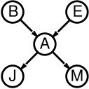
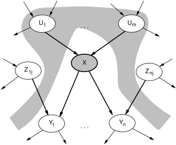
- Each node is conditionally independent of its nondescendants given its parents
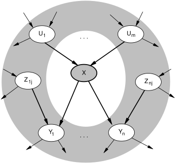
- Each node is conditionally independent of all others given its Markov blanket (parents + children + children’s parents)
Global semantics and Inference
The full joint distribution is defined as the product of the local conditional distributions: P(X_{1},\ldots,X_{n})=\prod_{i=1}^{n}P(X_{i}\mid parents(X_{i}))
- For example, \begin{align} P(j\land m\land a\land\lnot b\land\lnot e) & = & P(j\mid a)P(m\mid a)P(a\mid\lnot b,\lnot e)P(\lnot b)P(\lnot e)\\ & = & 0.9\times0.7\times0.001\times0.999\times0.998\\ & \approx & 0.00063 \end{align}
Learning
The Learning Problem
Known Structure |
Unknown Structure |
|
|---|---|---|
| Complete Data | Statistical parametric estimation (closed-form) | Discrete optimization over structures (discrete search) |
| Incomplete Data | Parametric optimization (EM, gradient descent...) | Combined (Structural EM, mixture models…) |
Learning problem includes
Parameter learning
Structure learning
Parameter Learning
Known Structure and Complete Data
Given a training data \mathcal{D}, find the best parameter {\color{red}\theta}s for multinomial variables \begin{equation} P_{{\color{red}\theta}}(X_{i}\mid pa_{i}) \end{equation} where pa_{i}=parents(X_{i}) (pa_{i} can be \emptyset)
Estimate parameter
Maximum likelihood \begin{equation} {\color{red}\hat{\theta}}_{{\color{red}ML}}=\frac{count(x_{i},pa_{i})}{count(pa_{i})} \end{equation} Maximum a posteriori \begin{equation} {\color{red}\hat{\theta}_{MAP}}=\frac{\alpha(x_{i},pa_{i})+count(x_{i},pa_{i})}{\alpha(pa_{i})+count(pa_{i})} \end{equation} where count(.) is the number of instances and \alpha(.) is the prior parameters.
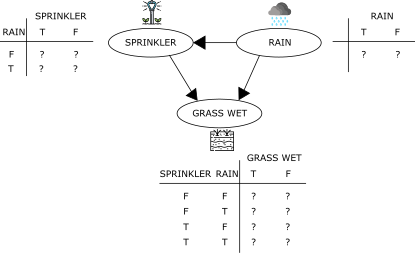
Example 4
Find the best parameter {\color{red}\theta}s given the following training data \mathcal{D}
# Rain Sprinkler Grass Wet 1 T T T 2 T T F 3 T F T 4 T F F 5 F T T 6 F T F 7 F F T 8 F F F 9 T T T 10 F T T 11 T F T 12 F F T 13 F T T 14 T T T
Structure Learning
Unknown Structure and Complete Data
- Need a method such that a series of locally testable assertions of conditional independence guarantees the required global semantics
Choose an ordering of variables X_{1},\ldots,X_{n}
For i = 1 to n
add X_{i} to the network
select parents from X_{1},\ldots,X_{i-1} such that
P(X_{i}\mid parents(X_{i}))=P(X_{i}\mid X_{1},\ldots,X_{i-1})
This choice of parents guarantees the global semantics:
\begin{array}{rcll} P(X_{1},\ldots,X_{n}) & = & \prod_{i=1}^{n}P(X_{i}\mid X_{1},\ldots,X_{i-1}) & (\text{chain rule})\\ & = & \prod_{i=1}^{n}P(X_{i}\mid parents(X_{i})) & (\text{by construction}) \end{array}
Example: Burglary alarm
Suppose we choose the ordering M, J, A, B, E
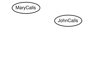
P(J\mid M)=P(J)?
Suppose we choose the ordering M, J, A, B, E
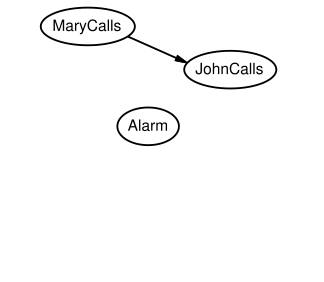
P(J\mid M)=P(J)? No
P(A\mid J,M)=P(A\mid J)? P(A\mid J,M)=P(A)?
Suppose we choose the ordering M, J, A, B, E
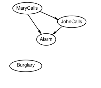
P(J\mid M)=P(J)? No
P(A\mid J,M)=P(A\mid J)? P(A\mid J,M)=P(A)? No
P(B\mid A,J,M)=P(B\mid A)?
P(B\mid A,J,M)=P(B)?
Suppose we choose the ordering M, J, A, B, E
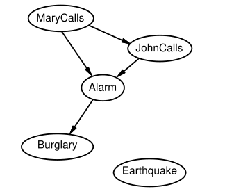
P(J\mid M)=P(J)? No
P(A\mid J,M)=P(A\mid J)? P(A\mid J,M)=P(A)? No
P(B\mid A,J,M)=P(B\mid A)? Yes
P(B\mid A,J,M)=P(B)? No
P(E\mid B,A,J,M)=P(E\mid A)?
P(E\mid B,A,J,M)=P(E\mid A,B)?
Suppose we choose the ordering M, J, A, B, E
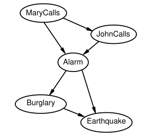
P(J\mid M)=P(J)? No
P(A\mid J,M)=P(A\mid J)? P(A\mid J,M)=P(A)? No
P(B\mid A,J,M)=P(B\mid A)? Yes
P(B\mid A,J,M)=P(B)? No
P(E\mid B,A,J,M)=P(E\mid A)? No
P(E\mid B,A,J,M)=P(E\mid A,B)? Yes
Deciding conditional independence is hard in noncausal directions (Causal models and conditional independence seem hardwired for humans!)
Assessing conditional probabilities is hard in noncausal directions
Network is less compact: 1+2+4+2+4=13 numbers needed
Examples
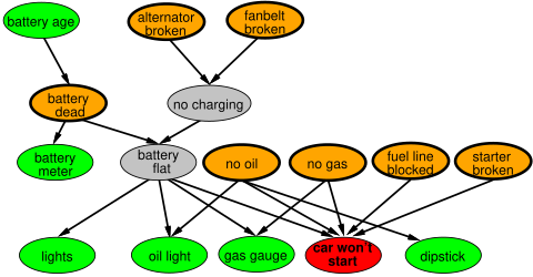
Example: Car diagnosis
Initial evidence (red): car won’t start
Testable variables (green), “broken, so fix it” variables (orange)
Hidden variables (gray) ensure sparse structure, reduce parameters
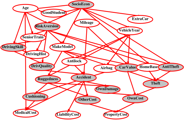
Example: Car insurance
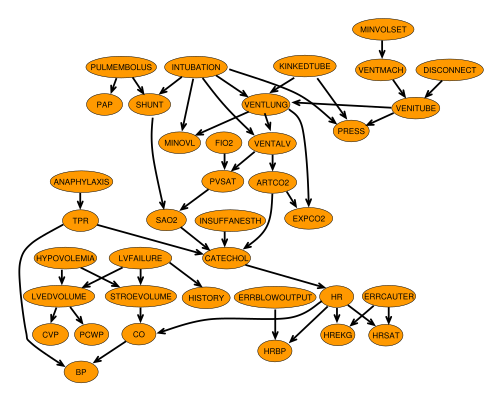
Example: “ICU Alarm” network
Domain: Monitoring Intensive-Care Patients
37 variables
509 parameters
More Representation
Compact distribution
Compact conditional distributions
Problem
CPT grows exponentially with number of parents
CPT does not work with continuous-valued parent or child
Deterministic nodes X: \begin{equation} X=f(parents(X))\text{ for some function }f \end{equation}
Boolean functions NorthAmerican=Canadian\lor US\lor Mexican
Numerical relationships among continuous variables \frac{\partial Level}{\partial t}=\text{ inflow + precipitation - outflow - evaporation}
Noisy-OR distributions model multiple noninteracting causes
Parents U_{1}\ldots U_{k} include all causes (can add leak node)
Independent failure probability q_{i} for each cause alone \begin{equation} P(X\mid U_{1}\ldots U_{j},\lnot U_{j+1}\ldots\lnot U_{k})=1-\prod_{i=1}^{j}q_{i} \end{equation} Number of parameters linear in number of parents
\begin{align*} \begin{array}{rcc} q_{cold} & = & P(\lnot fever\mid cold,\lnot flu,\lnot malaria)=0.6\\ q_{flu} & = & P(\lnot fever\mid\lnot cold,flu,\lnot malaria)=0.2\\ q_{malaria} & = & P(\lnot fever\mid\lnot cold,\lnot flu,malaria)=0.1 \end{array} \end{align*}
| Cold | Flu | Malaria | P(Fever) | P(\lnot Fever) |
|---|---|---|---|---|
| F | F | F | \textbf{0.0} | 1.0 |
| F | F | T | 0.9 | \textbf{0.1} |
| F | T | F | 0.8 | \textbf{0.2} |
| F | T | T | 0.98 | 0.02=0.2\times0.1 |
| T | F | F | 0.4 | \textbf{0.6} |
| T | F | T | 0.94 | 0.06=0.6\times0.1 |
| T | T | F | 0.88 | 0.12=0.6\times0.2 |
| T | T | T | 0.988 | 0.012=0.6\times0.2\times0.1 |
Continuous variable
Bayesian nets with continuous variables
Discrete (Subsidy? and Buys?); continuous (Harvest and Cost)
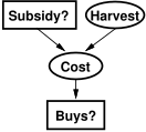
Option 1: discretization \to possibly large errors, large CPTs
Option 2: finitely parameterized canonical families
Continuous variable, discrete+continuous parents (e.g., Cost)
Discrete variable, continuous parents (e.g., Buys?)
Continuous child variables
Need one conditional density function for child variable given continuous parents, for each possible assignment to discrete parents
Most common is the linear Gaussian (LG) model, e.g.,: \begin{align} & & P(Cost=c\mid Harvest=h,Subsidy?=true)\\ & & =N(a_{t}h+b_{t},\sigma_{t})(c)=\frac{1}{\sigma_{t}\sqrt{2\pi}}\exp\left(-\frac{1}{2}\left(\frac{c-(a_{t}h+b_{t})}{\sigma_{t}}\right)^{2}\right) \end{align}
Mean Cost varies linearly with Harvest, variance is fixed
Linear variation is unreasonable over the full range but works OK if the likely range of Harvest is narrow
All-continuous network with LG distributions \implies full joint distribution is a multivariate Gaussian
Discrete+continuous LG network is a conditional Gaussian network i.e., a multivariate Gaussian over all continuous variables for each combination of discrete variable values
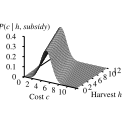
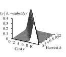
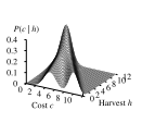
The graphs in (1) and (2) show the probability distribution over Cost as a function of Harvest size, with Subsidy true and false, respectively. Graph (3) shows the distribution P(Cost\mid Harvest), obtained by summing over the two subsidy cases.
Discrete variable given continuous parents
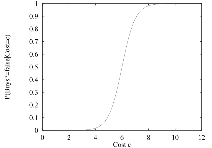
Probability of Buys? given Cost should be a “soft” threshold:
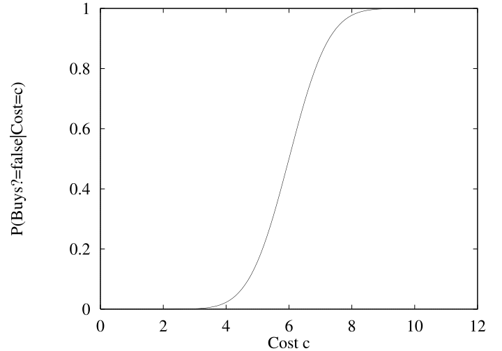
Probit distribution uses integral of Gaussian:
\Phi(x)=\int_{-\infty}^{x}\mathcal{N}(0,1)(x)dx
P(Buys?=true\mid Cost=c)=\Phi\left(\frac{-c+\mu}{\sigma}\right)
Sigmoid (or logit) distribution also used in neural networks: P(Buys?=true\mid Cost=c)=\frac{1}{1+\exp(-2\frac{-c+\mu}{\sigma})}
Sigmoid has similar shape to probit but much longer tails:
Why the probit/logit?
It’s sort of the right shape
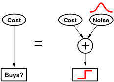
Can view as hard threshold whose location is subject to noise