7 PROBABILISTIC REASONING
Inference tasks
Optimal decisions: decision networks include utility information; probabilistic inference required for P(outcome\mid action,evidence)
Value of information: “which evidence to seek next?”
Sensitivity analysis: “which probability values are most critical?”
Explanation: “why do I need a new starter motor?”
7.1 Exact inference by enumeration
Inference by enumeration
Idea Slightly intelligent way to sum out variables from the joint without actually constructing its explicit representation
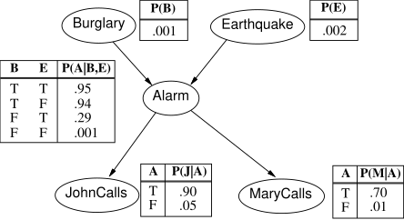
Simple query on the burglary network: \begin{array}{rcl} P(B\mid j,m) & = & P(B,j,m)/P(j,m)\\ & = & \alpha P(B,j,m)\\ & = & \alpha\sum_{e}\sum_{a}P(B,e,a,j,m) \end{array}
Rewrite full joint entries using product of CPT entries: \begin{array}{l} P(B\mid j,m)\\ =\alpha\:\sum_{e}\sum_{a}P(B)P(e)P(a\mid B,e)P(j\mid a)P(m\mid a)\\ =\alpha\:P(B)\sum_{e}P(e)\sum_{a}P(a\mid B,e)P(j\mid a)P(m\mid a)\\ =\alpha\:\left\langle 0.00059224,0.0014919\right\rangle \\ =\left\langle 0.284,0.716\right\rangle \end{array}
Evaluation tree
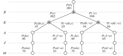
- Enumeration is inefficient: repeated computation; e.g., computes P(j\mid a)P(m\mid a) for each value of e
Enumeration algorithm
- Recursive depth-first enumeration: O(n) space, O(d^{n}) time
function Enumeration-Ask(X, \boldsymbol{e}, bn) returns a distribution over X
inputs: X, the query variable
\boldsymbol{e}, observed values for variables E
bn, a Bayes net with variables \{X\}\cup\boldsymbol{E}\cup\boldsymbol{Y} # \boldsymbol{Y}:hidden variables
Q(X) \gets a distribution over X, initially empty
for each value x_{i} of X do
Q(x_{i}) \gets Enumerate-All(bn.vars, \boldsymbol{e}_{x_{i}})
where \boldsymbol{e}_{x_{i}} is \boldsymbol{e} extended with X=x_{i}
return [Normalize][(Q(X))]
function Enumerate-All(vars, \boldsymbol{e}) returns a real number
if Empty?(vars) then return 1.0
Y \gets First(vars)
if Y has value y in \boldsymbol{e}
then return P(y\mid parents(Y)) \times Enumerate-All(Rest(vars), \boldsymbol{e})
else return \sum yP(y\mid parents(Y)) \times Enumerate-All(Rest(vars), \boldsymbol{e}_{y})
where \boldsymbol{e}_{y} is \boldsymbol{e} extended with Y=y
7.2 Exact inference by variable elimination
Inference by variable elimination
Idea Carry out summations right-to-left, storing intermediate results (factors) to avoid recomputation
\begin{align*} P(B\mid j,m) & =\alpha\:\underbrace{P(B)}_{B}\sum_{e}\underbrace{P(e)}_{E}\sum_{a}\underbrace{P(a\mid B,e)}_{A}\underbrace{P(j\mid a)}_{J}\underbrace{P(m\mid a)}_{M}\\ & =\alpha\:P(B)\sum_{e}P(e)\sum_{a}P(a\mid B,e)P(j\mid a)f_{M}(a)\\ & =\alpha\:P(B)\sum_{e}P(e)\sum_{a}P(a\mid B,e)f_{J}(a)f_{M}(a)\\ & =\alpha\:P(B)\sum_{e}P(e)\sum_{a}f_{A}(a,b,e)f_{J}(a)f_{M}(a)\\ & =\alpha\:P(B)\sum_{e}P(e)f_{\bar{A}JM}(b,e)\text{ (sum out A)}\\ & =\alpha\:P(B)f_{\bar{E}\bar{A}JM}(b)\text{ (sum out E)}\\ & =\alpha\:f_{B}(b)\times f_{\bar{E}\bar{A}JM}(b) \end{align*}
Variable elimination: Basic operations
Summing out a variable from a product of factors:
move any constant factors outside the summation
add up submatrices in pointwise product of remaining factors
\begin{align} \sum_{x}f_{1}\times\cdots\times f_{k} & =f_{1}\times\cdots\times f_{i}\sum_{x}\;f_{i+1}\times\cdots\times f_{k}\nonumber \\ & =f_{1}\times\cdots\times f_{i}\times f_{\bar{X}} \end{align}
assuming f_{1},\ldots,f_{i} do not depend on X
Pointwise product of factors f_{1} and f_{2}: \begin{equation} \begin{array}{l} f_{1}(x_{1},\ldots,x_{j},y_{1},\ldots,y_{k})\times f_{2}(y_{1},\ldots,y_{k},z_{1},\ldots,z_{l})\\ =f(x_{1},\ldots,x_{j},y_{1},\ldots,y_{k},z_{1},\ldots,z_{l}) \end{array} \end{equation}
Variable elimination algorithm
function Elimination-Ask(X, \boldsymbol{e}, bn)
returns a distribution over X
inputs: X, the query variable
\boldsymbol{e}, observed values for variables \boldsymbol{E}
bn, a Bayesian network specifying
joint distribution P(X_{1},\ldots,X_{n})
factors\gets\emptyset
for each var in Order(bn.\text{Vars}) do
factors\gets[\text{Make-Factor}(var,\boldsymbol{e})\mid factors]
if var is a hidden variable then
factors\gets\text{Sum-Out}(var,factors)
return Normalize(Pointwise-Product(factors))
Irrelevant variables
Consider the query P(JohnCalls\mid Burglary=true) P(J\mid b)=\alpha P(b)\sum_{e}P(e)\sum_{a}P(a\mid b,e)P(J\mid a)\sum_{m}P(m\mid a) Sum over m is identically 1; M is irrelevant to the query
Here, X=JohnCalls, \boldsymbol{E}=\{Burglary\}, and Ancestors(\{X\}\cup\boldsymbol{E})=\{Alarm,Earthquake\} so MaryCalls is irrelevant (Compare this to backward chaining from the query in Horn clause KBs)
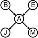
Y is irrelevant unless Y\in Ancestors(\{X\}\cup\boldsymbol{E})
Complexity of exact inference
Singly connected networks (or polytrees):
any two nodes are connected by at most one (undirected) path
time and space cost of variable elimination are O(d^{k}n)
Multiply connected networks:
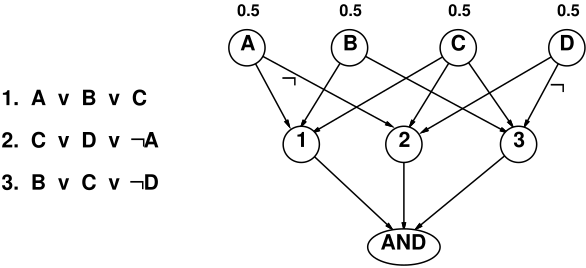
can reduce 3SAT to exact inference \implies NP-hard
equivalent to counting 3SAT models \implies P-complete
7.3 Approximate inference by stochastic simulation
Random Number
Uniform Random Numbers
The basis of all of these simulation methods is in the generation of random numbers
The simplest method is the linear congruential generator to generate uniformly distributed random numbers \begin{equation} x_{n+1}=(ax_{n}+c)\bmod m \end{equation} where a,c, and m are parameters that have to be chosen carefully, the initial input x_{0} is known as the seed
For example, we can use m=2^{32}, a=1,664,525 and c=1,013,904,223
Gaussian Random Numbers
Sampling for Single Categorical Variable
Want to sample values of a random variable X whose domain is {true, false}, with probability distribution
true false 0.4 0.6 Simple approach
r = uniform_random([0, 1])
if r < 0.4:
    sample = true
else:
    sample = false
Inference by stochastic simulation
Basic idea
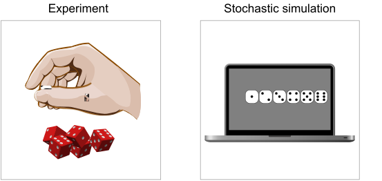
Draw N samples from a sampling distribution S (sampling is a lot like repeated simulation)
Compute an approximate posterior probability \hat{P}
Show this converges to the true probability P
Why sample?
Learning: get samples from a distribution you don’t know
Inference: getting a sample is faster than computing the right answer (e.g. with variable elimination)
Approaches:
Sampling from an empty network
Rejection sampling: reject samples disagreeing with evidence
Likelihood weighting: use evidence to weight samples
Markov chain Monte Carlo (MCMC): sample from a stochastic process whose stationary distribution is the true posterior
Direct Sampling
Sampling from an empty network
function Prior-Sample(bn)
returns an event sampled from the prior specified by bn
inputs: bn, a Bayesian network specifying
joint distribution P(X_{1},\ldots,X_{n})
\boldsymbol{x} \gets an event with n elements
foreach variable X_{i} in X_{1}, …, X_{n} do
\boldsymbol{x}[i] \gets a random sample from P(X_{i}\mid parents(X_{i}))
return \boldsymbol{x}
Example
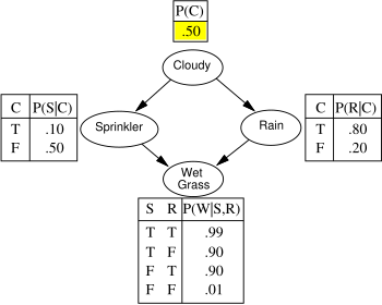
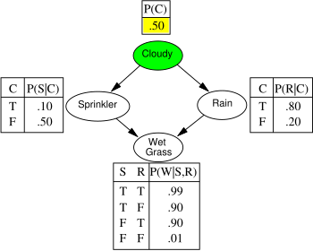
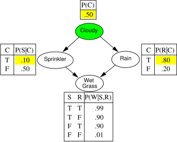
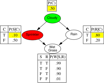
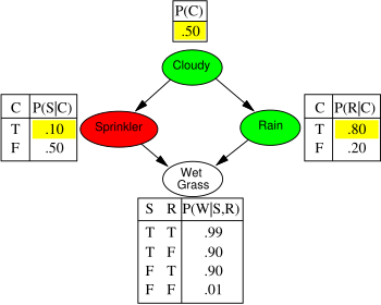
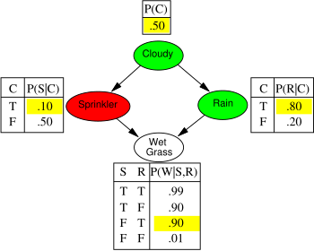
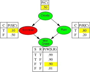
Estimate P(Cloudy,Sprinkler,Rain,WetGrass) using 100 samples
# Cloudy Sprinkler Rain Wet Grass 1 T F T T 2 T T T T 3 F T T F 4 T F T T 5 F F F T ... ... ... ... ... 100 T F T F
Analysis
Probability that PriorSample generates a particular event S_{PS}(x_{1}\ldots x_{n})=\prod_{i=1}^{n}P(x_{i}\mid Parents(x_{i}))=P(x_{1}\ldots x_{n})
Let N_{PS}(x_{1}\ldots x_{n}) be the number of samples generated for event x_{1},\ldots,x_{n}
Then we have \begin{align} \lim_{N\to\infty}\hat{P}(x_{1},\ldots,x_{n}) & = & \lim_{N\to\infty}N_{PS}(x_{1},\ldots,x_{n})/N\\ & = & S_{PS}(x_{1},\ldots,x_{n})=P(x_{1}\ldots x_{n}) \end{align} That is, estimates derived from PriorSample are consistent
Rejection Sampling
Rejection sampling
- \hat{P}(X\mid e) estimated from samples agreeing with e
function Rejection-Sampling(X, e, bn, N)
returns an estimate of P(X\mid e)
inputs: X, the query variable
e, observed values for variables E
bn, a Bayesian network
N, the total number of samples to be generated
local variables: \boldsymbol{N}, a vector of counts for each value of X,
initially zero
for j = 1 to N do
x \gets Prior-Sample(bn)
if x is consistent with e then
N[x]\gets N[x]+1 where x is the value of X in x
return Normalize(N)
Exampe
Estimate P(Rain\mid Sprinkler=true) using 100 samples
Results 27 samples have Sprinkler=true; of these, 8 have Rain=true and 19 have Rain=false.
# Cloudy Sprinkler Rain Wet Grass 1 T F T T 2 T T T T 3 F T T F 4 T F T T 5 F F F T ... ... ... ... ... 100 T F T F
\;\to\;
| # | Sprinkler | Rain |
|---|---|---|
| 1 | T | T |
| 2 | T | T |
| 3 | T | T |
| 4 | T | F |
| 5 | T | T |
| ... | ... | ... |
| 27 | T | F |
Analysis of rejection sampling
| \hat{P}(X\mid e) | = | \alpha N_{PS}(X,e) | (algorithm defn.) |
| = | N_{PS}(X,e)/N_{PS}(e) | (normalized by N_{PS}(e)) | |
| \approx | P(X,e)/P(e) | (property of PriorSample) | |
| = | P(X\mid e) | (defn. of conditional probability) |
Hence rejection sampling returns consistent posterior estimates
Problem: hopelessly expensive if P(e) is small. P(e) drops off exponentially with number of evidence variables!
Likelihood Weighting
Likelihood weighting
- Idea: fix evidence variables, sample only nonevidence variables, and weight each sample by the likelihood it accords the evidence
function Likelihood-Weighting(X, e, bn, N) returns an estimate of P(X\mid e)
inputs: X, the query variable
e, observed values for variables E
bn, a Bayesian network specifying joint distribution P(X_{1},\ldots,X_{n})
N, the total number of samples to be generated
local variables: W, a vector of weighted counts for each value of X, initially zero
for j = 1 to N do
x,w\gets\text{Weighted-Sample}(bn,e)
W[x]\gets W[x]+w where x is the value of X in x
return Normalize(W)
function Weighted-Sample(bn, e) returns an event and a weight
w\gets1
x \gets an event with n elements initialized from e
foreach variable X_{i} in X_{1},\ldots,X_{n} do
if X_{i} is an evidence variable with value x_{i} in e
then w\gets w\times P(X_{i}=x_{i}\mid parents(X_{i}))
else x[i] \gets a random sample from P(X_{i}\mid parents(X_{i}))
return x, w
Likelihood weighting example
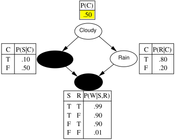
w=1.0
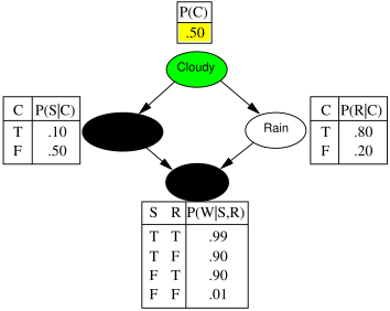
w=1.0
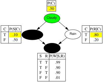
w=1.0
w=1.0\times0.1
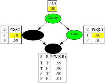
w=1.0\times0.1
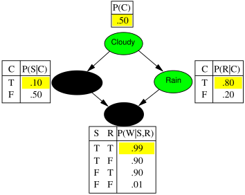
w=1.0\times0.1
w=1.0\times0.1\times0.99=0.099
Estimate P(Rain\mid Sprinkler=true,WetGrass=true) using 100 samples
# Cloudy Sprinkler Rain Wet Grass weight w 1 T T T T 0.099 2 F T T T ... 3 T T T T ... 4 F T T T ... 5 T T F T ... ... ... ... ... ... ... 100 F T T T ...
Likelihood weighting analysis
Sampling probability for WeightedSample is S_{WS}(z,e)=\prod_{i=1}^{l}P(z_{i}\mid parents(Z_{i}))
Note: pays attention to evidence in ancestors only \implies somewhere “in between” prior and posterior distribution
Weight for a given sample z,e is w(z,e)=\prod_{i=1}^{m}P(e_{i}\mid parents(E_{i}))
Weighted sampling probability is
S_{WS}(z,e)w(z,e) =\prod_{i=1}^{l}P(z_{i}\mid parents(Z_{i}))\prod_{i=1}^{m}P(e_{i}\mid parents(E_{i})) =P(z,e) (by standard global semantics of network) Hence likelihood weighting returns consistent estimates but performance still degrades with many evidence variables because a few samples have nearly all the total weight
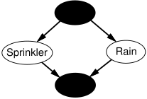
7.4 Approximate inference by Markov chain Monte Carlo (MCMC)
Gibbs Sampling
State
State \boldsymbol{x} is current assignment to all variables.
Transition probability q(\boldsymbol{x}\to\boldsymbol{x}') is the probability to change from state \boldsymbol{x} to \boldsymbol{x}'
Occupancy probability \pi_{t}(\boldsymbol{x}) is the probability in state \boldsymbol{x} at time t
Stationary distribution
\pi_{t}(\boldsymbol{x}) = probability in state \boldsymbol{x} at time t
\pi_{t+1}(\boldsymbol{x}') = probability in state \boldsymbol{x}' at time t+1
\pi_{t+1} in terms of \pi_{t} and q(\boldsymbol{x}\to\boldsymbol{x}') \begin{equation} \pi_{t+1}(q(\boldsymbol{x}\to\boldsymbol{x}')')=\sum_{\boldsymbol{x}}\pi_{t}(\boldsymbol{x})q(\boldsymbol{x}\to\boldsymbol{x}') \end{equation}
Stationary distribution: \pi_{t}=\pi_{t+1}=\pi \begin{equation} \pi(\boldsymbol{x}')=\sum_{\boldsymbol{x}}\pi(\boldsymbol{x})q(\boldsymbol{x}\to\boldsymbol{x}')\text{ for all }\boldsymbol{x}' \end{equation}
- If \pi exists, it is unique (specific to q(\boldsymbol{x}\to\boldsymbol{x}'))
Detailed balance
Detailed balance: “Outflow” = “inflow” for each pair of states: \begin{equation} \pi(\boldsymbol{x})q(\boldsymbol{x}\to\boldsymbol{x}')=\pi(\boldsymbol{x}')q(\boldsymbol{x}'\to\boldsymbol{x})\text{ for all }\boldsymbol{x},\boldsymbol{x}' \end{equation}
Detailed balance \implies stationarity:
\begin{align} \sum_{\boldsymbol{x}}\pi(\boldsymbol{x})q(\boldsymbol{x}\to\boldsymbol{x}') & = & \sum_{\boldsymbol{x}}\pi(\boldsymbol{x}')q(\boldsymbol{x}'\to\boldsymbol{x})\\ & = & \pi(\boldsymbol{x}')\sum_{\boldsymbol{x}}q(\boldsymbol{x}'\to\boldsymbol{x})\\ & = & \pi(\boldsymbol{x}') \end{align}
Gibbs sampling
MCMC algorithms typically constructed by designing a transition probability q that is in detailed balance with desired \pi
Sampling X_{i}, let \bar{\boldsymbol{X}_{i}} be all other nonevidence variables
Current values are x_{i} and \bar{\boldsymbol{x}_{i}}; \boldsymbol{e} is fixed
Transition probability is given by q(\boldsymbol{x}\to\boldsymbol{x}')=q(x_{i},\bar{\boldsymbol{x}}_{i}\to x_{i}',\bar{\boldsymbol{x}}_{i})=P(x_{i}'\mid\bar{\boldsymbol{x}}_{i},\boldsymbol{e}) This gives detailed balance with true posterior P(\boldsymbol{x}\mid\boldsymbol{e}): \begin{align} \pi(\boldsymbol{x})q(\boldsymbol{x}\to\boldsymbol{x}') & = & P(\boldsymbol{x}\mid\boldsymbol{e})P(x_{i}'\mid\bar{\boldsymbol{x}_{i}},\boldsymbol{e})=P(x_{i},\bar{\boldsymbol{x}_{i}}\mid\boldsymbol{e})P(x_{i}'\mid\bar{\boldsymbol{x}_{i}},\boldsymbol{e})\\ & = & P(x_{i}\mid\bar{\boldsymbol{x}_{i}},\boldsymbol{e})P(\bar{\boldsymbol{x}_{i}}\mid\boldsymbol{e})P(x_{i}'\mid\bar{\boldsymbol{x}_{i}},\boldsymbol{e})\text{ (chain rule)}\\ & = & P(x_{i}\mid\bar{\boldsymbol{x}_{i}},\boldsymbol{e})P(x_{i}',\bar{\boldsymbol{x}_{i}}\mid\boldsymbol{e})\text{ (chain rule backwards)}\\ & = & q(\boldsymbol{x}'\to\boldsymbol{x})\pi(\boldsymbol{x}')\\ & = & \pi(\boldsymbol{x}')q(\boldsymbol{x}'\to\boldsymbol{x}) \end{align}
Analysis
Chain approaches stationary distribution: long-run fraction of time spent in each state is exactly proportional to its posterior probability
Gibbs sampling transition probability: sample each variable given current values of all others \implies detailed balance with the true posterior
For Bayesian networks, Gibbs sampling reduces to sampling conditioned on each variable’s Markov blanket
Performance of approximation algorithms
Absolute approximation: \mid P(X\mid\boldsymbol{e})-\hat{P}(X\mid\boldsymbol{e})\mid\leq\epsilon
Relative approximation: \frac{\mid P(X\mid\boldsymbol{e})-\hat{P}(X\mid\boldsymbol{e})\mid}{P(X\mid\boldsymbol{e})}\leq\epsilon
Relative \implies absolute since 0\leq P\leq1 (may be O(2^{-n}))
Randomized algorithms may fail with probability at most \delta
Polytime approximation: \text{poly}(n,\epsilon^{-1},\log\delta^{-1})
Both absolute and relative approximation for either deterministic or randomized algorithms are NP-hard for any \epsilon,\delta<0.5 (absolute approximation polytime with no evidence—Chernoff bounds)
MCMC for Bayesian Network
Approximate inference using MCMC
“State” of network = current assignment to all variables.
function Mcmc-Ask(X, e, bn, N)
returns an estimate of P(X\mid e)
local variables: N, a vector of counts for each value of X,
initially zero
Z, the nonevidence variables in bn
x, the current state of the network,
initially copied from e
initialize x with random values for the variables in Z
for j = 1 to N do
for each Z_{i} in Z do
set the value of Z_{i} in x by sampling from P(Z_{i}\mid mb(Z_{i}))
N[x]\gets N[x]+1 where x is the value of X in x
return Normalize(N)
The Markov chain
- With Sprinkler=true,WetGrass=true, there are four states:
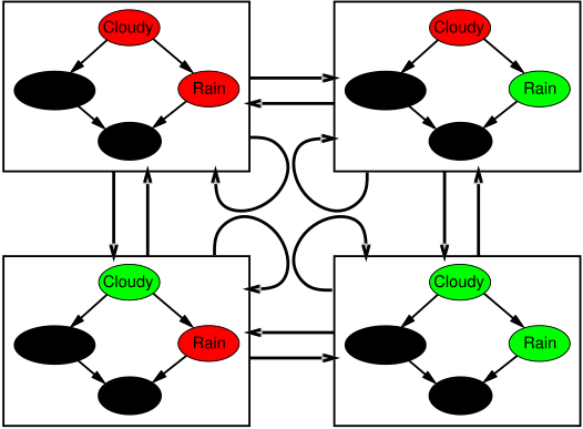
- Wander about for a while, average what you see
MCMC example
Estimate P(Rain\mid Sprinkler=true,WetGrass=true)
Sample Cloudy or Rain given its Markov blanket, repeat.
Count number of times Rain is true and false in the samples.
Result: visit 100 states, 31 have Rain=true, 69 have Rain=false

| # | Cloudy | Sprinkler | Rain | Wet Grass |
|---|---|---|---|---|
| 1 | T | T | T | T |
| 2 | F | T | T | T |
| 3 | F | T | T | T |
| 4 | F | T | F | T |
| ... | ... | ... | ... | ... |
| 100 | T | T | F | T |
Markov blanket sampling
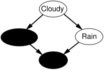
Markov blanket of Cloudy is Sprinkler and Rain
Markov blanket of Rain is Cloudy, Sprinkler, and WetGrass
- Probability given the Markov blanket is calculated as follows:
P(x_{i}'\mid mb(X_{i}))=P(x_{i}'\mid parents(X_{i}))\prod_{Z_{j}\in children(X_{i})}P(z_{j}\mid parents(Z_{j}))
Easily implemented in message-passing parallel systems
Main computational problems:
Difficult to tell if convergence has been achieved
Can be wasteful if Markov blanket is large: P(X_{i}\mid mb(X_{i})) won’t change much (law of large numbers)
7.5 Sampling for Continous Variables
Reject Sampling
Reject Sampling
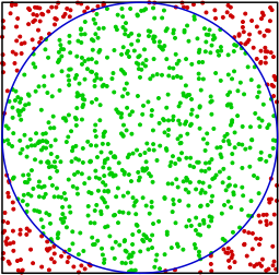
\pi\approx4\times\frac{\text{number of points inside circle}}{\text{number of points inside square}}
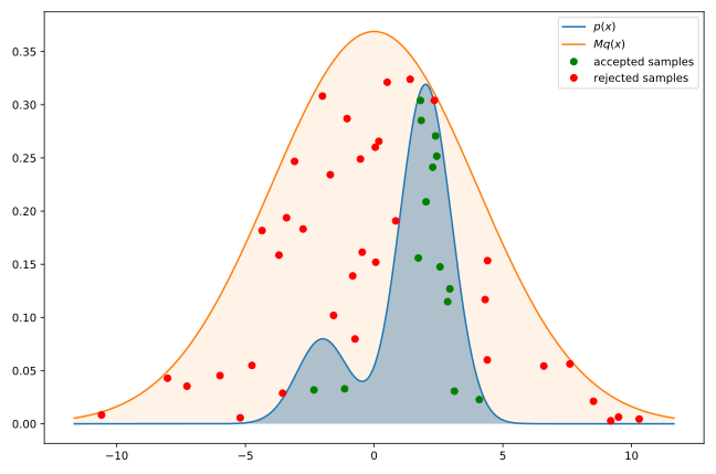
p(x) is a target distribution, q(x) is an an easy-to-sample distribution and M is a constant such that \forall x\in\mathcal{X},p(x)\leq Mq(x)
Metropolis-Hastings
Metropolis-Hastings algorithm
Choose an initial value for a sample x_{0}
Propose a new sample value x_{i+1} given x_{i} from q(x\mid x_{i})
Compute the probability of accepting a new parameter value by using the Metropolis-Hastings criteria: \begin{equation} \rho=\min\left(1,\frac{p(x_{i+1})}{p(x_{i})}\right) \end{equation}
Sample u from a \mathcal{U}[0,1]
If u<\rho we accept the new value x_{i+1}; otherwise, we stay in the old value x_{i}
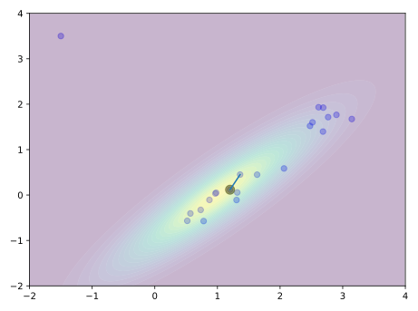
Example