11 ENSEMBLE MODEL
Big Picture

11.1 Ensemble Model
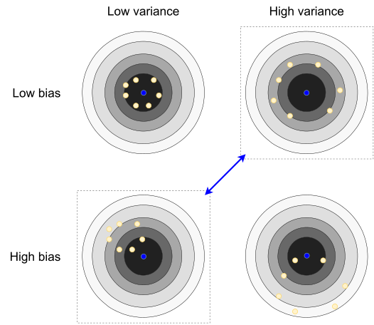
Bias vs. Variance
- Low-bias models tend to have high variance, and vice versa.
Basics of Ensembles
Instead of providing one model, an ensemble approach proposes many models to the same problem, and combine them
- The simplest ensemble H over models \{h_{i}\in\mathcal{H},i=1...T\} \begin{equation} H(\boldsymbol{x})=\sum_{i=1}^{T}{\color{red}\alpha_{i}}h_{i}(\boldsymbol{x})\text{ with }\sum_{i=1}^{T}{\color{red}\alpha_{i}}=1 \end{equation}
Why should this be a good idea?
- combine models \to reduce the variance \to enhance expected performance.
However, increase the performance cost
Why Does it Work?
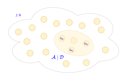
It has been shown that the expected risk of the average of a set of models is better than the average of the expected risk of these models
Let us consider the simplest ensemble H over models h_{i} \begin{equation} H(\boldsymbol{x})=\sum_{i=1}^{T}{\color{red}\alpha_{i}}h_{i}(\boldsymbol{x})\text{ with }\sum_{i=1}^{T}{\color{red}\alpha_{i}}=1 \end{equation}
The MSE risk of h_{i} at \boldsymbol{x} is \begin{equation} e_{i}(\boldsymbol{x})=\mathbb{E}_{y}[(y-h_{i}(\boldsymbol{x}))^{2}] \end{equation}
The average risk \bar{e}(\boldsymbol{x}) of a model is \begin{equation} \bar{e}(\boldsymbol{x})=\sum_{i}{\color{red}\alpha_{i}}e_{i}(\boldsymbol{x}) \end{equation}
The average risk e(\boldsymbol{x}) of the ensemble is \begin{equation} e(\boldsymbol{x})=\mathbb{E}_{y}[(y-H(\boldsymbol{x}))^{2}] \end{equation}
Let us define diversity \begin{equation} d_{i}(\boldsymbol{x})=(h_{i}(\boldsymbol{x})-H(\boldsymbol{x}))^{2} \end{equation}
The average diversity is \begin{equation} \bar{d}(\boldsymbol{x})=\sum_{i}{\color{red}\alpha_{i}}d_{i}(\boldsymbol{x}) \end{equation}
It can then be shown that \begin{align} e(\boldsymbol{x}) & =\bar{e}(\boldsymbol{x})-\bar{d}(\boldsymbol{x})\\ e(\boldsymbol{x}) & <\bar{e}(\boldsymbol{x}) \end{align}
11.2 Bagging
Bagging
Underlying idea A part of the variance is due to the specific choice of the training data set
Let us create many similar training data sets,
For each of them, let us train a new function f_{i}
The final function will be the average of each function outputs.
- How similar? using bootstrap aggregating
Bootstrap
Bootstrap
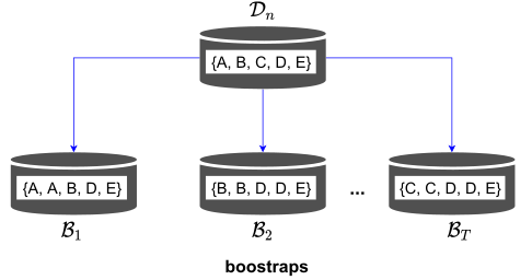
Given a data set \mathcal{D}_{n} with n examples drawn from p(\mathcal{Z})=p(\mathcal{X},\mathcal{Y}), a bootstrap \mathcal{B}_{i},i=1...T of \mathcal{D}_{n} also contains n examples:
for j=1\to n
the j-th example of B_{i} is drawn independently with replacement from \mathcal{D}_{n}
Some examples from \mathcal{D}_{n} are in multiple copies in \mathcal{B}_{i}
Some examples from \mathcal{D}_{n} are not in \mathcal{B}_{i}
The examples were i.i.d. drawn from p(Z) \to the datasets \mathcal{B}_{i} are as plausible as \mathcal{D}_{n}, but drawn from \mathcal{D}_{n} instead of p(Z).
Algorithm
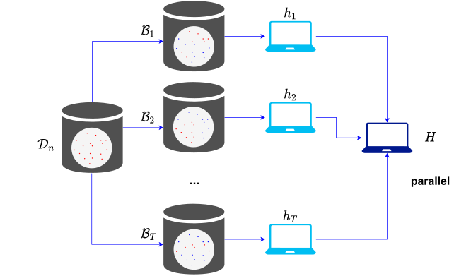
Diagram
Algorithm
Training:
Given a training set \mathcal{D}_{n}, create T bootstraps \mathcal{B}_{i} of \mathcal{D}_{n}
For each bootstrap \mathcal{B}_{i}, select \begin{equation} h_{i}=\arg\min_{h\in\mathcal{H}}E(h\mid\mathcal{B}_{i}) \end{equation}
Running:
- Given an input \boldsymbol{x}, the corresponding output \hat{y} is: \begin{equation} \hat{y}=H(\boldsymbol{x})=\frac{1}{T}\sum_{i=1}^{T}h_{i}(\boldsymbol{x}) \end{equation}
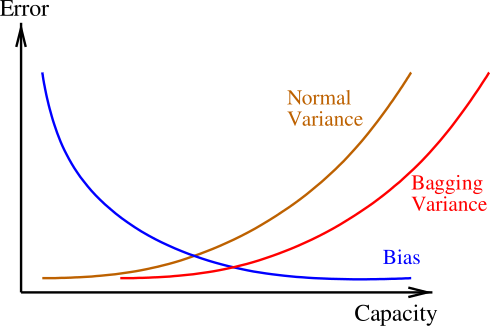
Bias + Variance
- Analysis: if generalization error is decomposed into bias and variance terms then bagging reduces variance.
Random Forests
Random Forests
A random forest is an ensemble of decision trees.
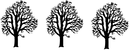
Each decision tree h_{i} is trained as follows:
Create a bootstrap of the training set
Select a subset m\ll d input variables as potential split nodes (m is constant over all trees)
No pruning of the trees
A decision is taken by voting amongst the trees
- Somehow, m controls the capacity.
11.3 Boosting
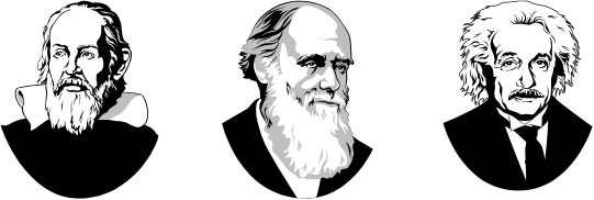
Big Picture
Diagram
Weak vs. Strong Learning Model
A learning model is strong iff every hypothesis h has low error
A learning model is weak iff every hypothesis h has high error
Examples of weak classifiers:
Simple decision trees such as stumps
Simple neural networks such as perceptrons
Haar-like features
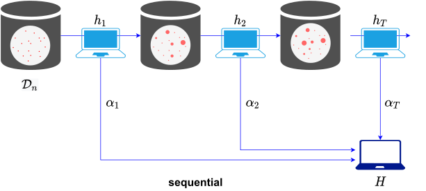
Boosting
Boosting involves three elements:
A loss function to be optimized \ell(.,.)
A set of weak learners \{h_{t}(x)\}
An additive model H(x) to add weak learners to minimize the loss function \begin{equation} H(x)=\sum_{t=1}^{T}{\color{red}\alpha_{t}}h_{t}(x) \end{equation}
Loss function
Square loss \begin{equation} \ell(\hat{y},y)=(\hat{y}-y)^{2} \end{equation}
Absolute loss \begin{equation} \ell(\hat{y},y)=|\hat{y}-y| \end{equation}
Huber loss \begin{equation} \ell(\hat{y},y)=\begin{cases} \frac{1}{2}(\hat{y}-y)^{2} & (\hat{y}-y)\leq\delta\\ \delta(|\hat{y}-y|-\delta/2) & (\hat{y}-y)>\delta \end{cases} \end{equation}
Exponential loss \begin{equation} \ell(\hat{y},y)=e^{-\hat{y}\,y} \end{equation}
AdaBoost
AdaBoost
AdaBoost, short for Adaptive Boosting, is the most popular algorithm in the family of boosting algorithms
Simplest framework: binary classification H(x)
Simplest requirement: each weak classifier y=h_{t}(x), y\in\left\{ -1,+1\right\} should perform better than chance
Loss function: \begin{equation} \ell((H(x),y))=e^{-yH(x)} \end{equation}
Algorithm
Inputs: training data \mathcal{D}=\left\{ (\boldsymbol{x}_{1},y_{1}),\cdots,(\boldsymbol{x}_{N},y_{N})\right\} and a set of weak binary classifiers \left\{ h_{i}\in\mathcal{H}\right\}
Initialize the weights’ distribution of training data \begin{equation} (w_{1}^{(1)},w_{2}^{(1)},\cdots,w_{N}^{(1)})=\left(\frac{1}{N},\frac{1}{N},\cdots,\frac{1}{N}\right) \end{equation}
Iterate over t=1,2,\dotsc,T, use training data with current weights’ distribution
Find a weak classifier h_{t}(\boldsymbol{x}) that that minimizes the error rate e_{t} of over the training data \begin{equation} e_{t}=P(h_{t}(\boldsymbol{x}_{i})\neq y_{i})=\sum_{i=1}^{N}w_{i}^{(t)}\mathbb{I}(h_{t}(\boldsymbol{x}_{i})\neq y_{i}) \end{equation}
Compute the weight of classifier h_{t}(\boldsymbol{x}) \begin{equation} {\color{red}\alpha_{t}}=\frac{1}{2}\log\frac{1-e_{t}}{e_{t}} \end{equation}
Update the weights’ distribution of training data \begin{equation} w_{i}^{(t+1)}=w_{i}^{(t)}\exp(-{\color{red}\alpha_{t}}y_{i}h_{t}(\boldsymbol{x}_{i})) \end{equation}
Normalize the weights of data points \begin{equation} w_{i}=\frac{w_{i}}{\sum_{i}w_{i}} \end{equation}
Ensemble T weak classifiers \begin{equation} \text{sign}\left[H(\boldsymbol{x})\right]=\text{sign}\left[\sum_{t=1}^{T}{\color{red}\alpha_{t}}h_{t}(\boldsymbol{x})\right] \end{equation}
Example
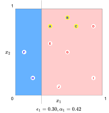
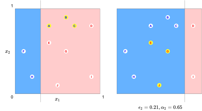
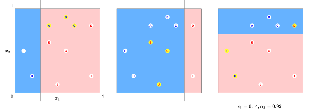
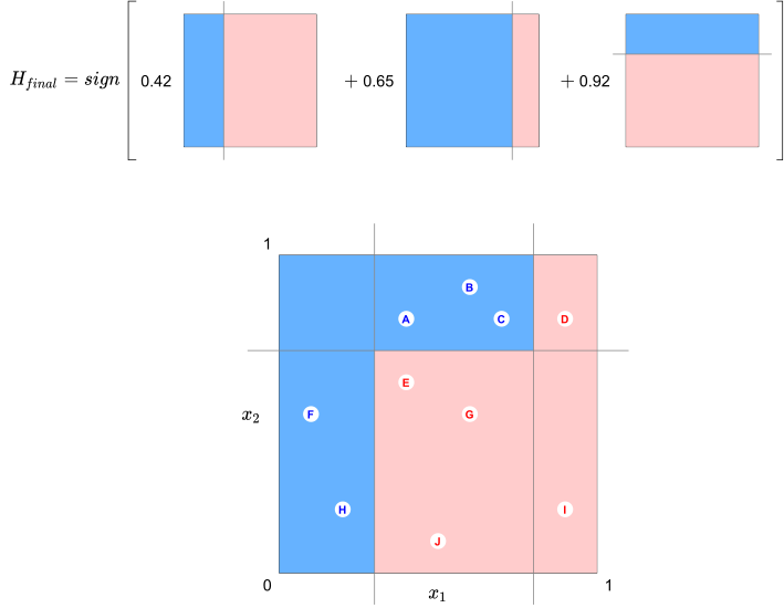
Given a training data set \mathcal{D}= {A, B, C, D, E, F, G, H, I, J}, find a strong classifier from weak classifiers (vertical or horizontal lines)
# x_{1} x_{2} label A 0.4 0.8 1 B 0.6 0.9 1 C 0.7 0.8 1 D 0.9 0.8 -1 E 0.4 0.6 -1 F 0.1 0.5 1 G 0.6 0.5 -1 H 0.2 0.2 1 I 0.9 0.2 -1 J 0.5 0.1 -1
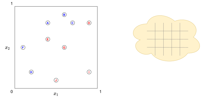
Round 1
Round 2
Round 3
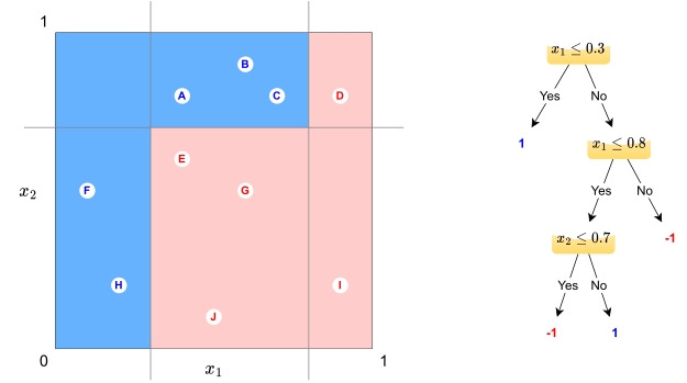
The combined classifier
Tree based classifier
Analysis
Selection of {\color{red}\alpha_{t}} comes from minimizing \begin{equation} \arg\min_{{\color{red}\alpha_{t}}}\sum_{i=1}^{N}\exp\left(-y_{i}\left[H_{t-1}(\boldsymbol{x}_{i})+{\color{red}\alpha_{t}}h_{t}(\boldsymbol{x}_{i})\right]\right) \end{equation}
If each weak classifier is always better than chance, then AdaBoost can be proven to converge to 0 training error
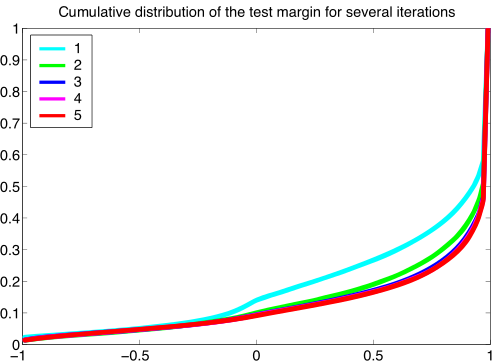
Even after training error is 0, generalization error continues to improve: the margin continues to grow
Sampling can often be replaced by weighting
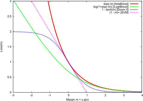
Cost Functions
- Comparison of various cost functions related to AdaBoost
Margin
- The AdaBoost margin is defined as the distribution of y\cdot h(x)
Face Detection
Face Detection
Face detection framework was proposed in 2001 by Paul Viola and Michael Jones using AdaBoost
- Some hypotheses h_{\theta}
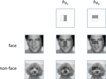
- Haar-like features for each hypothesis
\begin{equation} h_{\theta}=\sum_{(x,y)\in\text{dark area}}image(x,y)-\sum_{(x,y)\in\text{white area}}image(x,y) \end{equation}
Gradient Boosting
What is Gradient Boosting
Gradient Boosting = Gradient Descent + Boosting
In Adaboost, “losses” are identified by high-weight data points
In Gradient Boosting, “losses” are identified by gradients
Gradient Boosting can be applied for different problems
Regression \to Classification \to Ranking
Algorithm
Input: training set \left\{ (x_{i},y_{i})\right\} _{i=1}^{n} and a differentiable loss function \ell(y,H(x)), number of iterations M.
Initialize model with a constant value: \begin{equation} H_{0}(x)={\color{red}\gamma}_{{\color{red}0}}=\arg\min_{{\color{red}\gamma}}\sum_{i=1}^{n}\ell(y_{i},{\color{red}\gamma}). \end{equation}
For m=1 to M:
Compute so-called pseudo-residuals: \begin{equation} r_{im}=-\left[\frac{\partial\ell(y_{i},H(x_{i}))}{\partial H(x_{i})}\right]_{H(x)=H_{m-1}(x)},\text{ for }i=1,...,m \end{equation}
Fit a base learner (or weak learner, e.g. tree) closed under scaling h_{m}(x) to pseudo-residuals, i.e. train it using the training set \left\{ (x_{i},r_{im})\right\} _{i=1}^{n}.
Compute multiplier by solving the following one-dimensional optimization problem: \begin{equation} {\color{red}\gamma_{m}}=\arg\min_{{\color{red}\gamma}}\sum_{i=1}^{n}\ell\left(y_{i},H_{m-1}(x_{i})+{\color{red}\gamma}h_{m}(x_{i})\right). \end{equation}
Update the model: \begin{equation} H_{m}(x)=H_{m-1}(x)+{\color{red}\gamma_{m}}h_{m}(x) \end{equation}
Output H_{M}(x)
Important points to remember
Bagging is predominantly a variance-reduction technique, while boosting is primarily a bias-reduction technique.
This explains why bagging is often used in combination with high-variance models such as tree models, whereas boosting is typically used with high-bias models such as linear classifiers.