9 FEATURE SELECTION AND REPRESENTATION
9.1 Motivation
Why Should We Select Features?
Some problems are defined by 100 or even 1000 input features
Most Machine Learning models have to attribute parameters to handle these features (often at least linearly as much)
Hence, capacity is determined by the number of features
If most features are noise, then most of the parameters will be useless \to capacity is wasted
Worse, the algorithm might find false regularities in the input features of the training data and use the wasted capacity to represent them!
Other problem: curse of dimensionality.
Finally: for more interpretability and efficiency.
Classes of Feature Selection Methods
Broad classes of feature selection methods:
Filter Methods:
Select the best features according to a reasonable criterion
The criterion is independent of the real problem
Wrapper Methods:
Select the best features according to the final criterion
For each subset of features, try to solve the problem
In any case, there are \sum_{p=1}^{N}\binom{p}{N}=\sum_{p=1}^{N}\frac{N!}{p!(N-p)!}\text{ \textbf{combinations}}
Alternative: weighting methods.
9.2 Filters
Filter Methods
Basic idea: select the best features according to some prior knowledge
Examples of prior knowledge:
if we accept to transform the features...
features should be uncorrelated \to perform a PCA and keep only the eigenvectors corresponding to x% of the variance.
similar ideas: linear discriminant analysis (LDA), independent component analysis (ICA)
features should have strong correlation with the target \to select the k features most linearly correlated to the target
select the k features with highest mutual information with the target:
I(x,y)=\sum_{i}\sum_{j}p(x=i,y=j)\log\left[\frac{p(x=i,y=j)}{p(x=i)p(y=j)}\right]
9.3 Wrappers
Wrapper Methods
Basic (naive) algorithm:
For each subset of features, solve the problem.
Select the best subset.
Impossible because the problem is exponentially long!
Alternatives: greedy heuristics such as forward selection or backward elimination
Forward Selection
let \mathcal{P}=\emptyset be the current set of selected features
let \mathcal{Q} be the full set of features
while size of \mathcal{P} smaller than a given constant
for each v\in\mathcal{Q}
set \mathcal{P}'\gets\left\{ v\right\} \cup\mathcal{P}
train the model with \mathcal{P}' and keep the validation performance
set \mathcal{P}'\gets\left\{ v^{\ast}\right\} \cup\mathcal{P} where v^{\ast} corresponds to the best validation performance obtained in step 3.1
set \mathcal{Q}\gets\mathcal{Q}\backslash\left\{ v^{\ast}\right\}
keep the validation performance obtained with current \mathcal{P}
return the best set \mathcal{P}
Backward Elimination
let \mathcal{P} be the full set of features
while size of \mathcal{P} smaller than a given constant
for each v\in\mathcal{P}
set \mathcal{P}'\gets\mathcal{P}\backslash\left\{ v\right\}
train the model with \mathcal{P}' and keep the validation performance
set \mathcal{P}'\gets\mathcal{P}\backslash\left\{ v^{\ast}\right\} where v^{\ast} corresponds to the worst validation performance obtained in step 2.1
keep the validation performance obtained with current \mathcal{P}
return the best set \mathcal{P}
9.4 Feature Weighting
Feature Weighting Methods
Instead of selecting a subset of features, which is a combinatorial problem, why not simply weight them?
Most feature weighting methods are based on the wrapper approach
Heuristics for feature weighting:
gradient descent on the input space \to train with all features, then fix the parameters and estimate the importance of each input, and loop
AdaBoost when each model is trained on one feature only (\to final solution is a linear combination)
9.5 Principal Component Analysis
Introduction
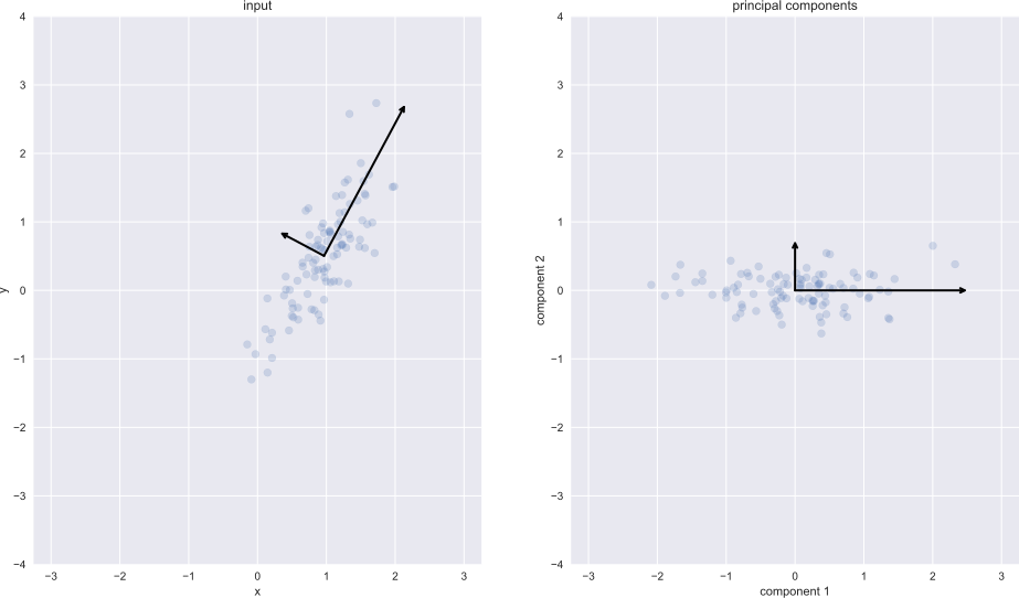
Principal Component Analysis (PCA) is an unsupervised dimension-reduction tool that can be used to reduce a large set of variables to a small set that still contains most of the information in the large set.
Algorithm
Input: Data \mathcal{D}=\{\boldsymbol{x}_{1},...,\boldsymbol{x}_{n}\},\boldsymbol{x}_{i}\in\mathbb{R}^{D}
Output: projection matrix W
Construct the mean vector \boldsymbol{\mu} \boldsymbol{\mu}=\frac{1}{n}\sum_{i=1}^{n}\boldsymbol{x}_{i}
Construct the covariance matrix S. S=\frac{1}{n}\sum_{i=1}^{n}(\boldsymbol{x}{}_{i}-\boldsymbol{\mu}_{i})(\boldsymbol{x}_{i}-\boldsymbol{\mu}_{i})^{\intercal}
Decompose the covariance matrix into its eigenvectors and eigenvalues. \{\boldsymbol{w}_{1},...,\boldsymbol{w}_{D}\}\text{ and }\{\lambda_{1},...,\lambda_{D}\}
Sort the eigenvalues by decreasing order to rank the corresponding eigenvectors. \{\boldsymbol{w}_{1},...,\boldsymbol{w}_{D}\}\text{ where }\lambda_{1}\geq...\geq\lambda_{D}
Select k eigenvectors which correspond to the k largest eigenvalues, where k is the dimensionality of the new feature subspace (k\leq D). \{\boldsymbol{w}_{1},...,\boldsymbol{w}_{k}\}\text{ where }\lambda_{1}\geq...\geq\lambda_{k}
Construct a projection matrix W from the “top” k eigenvectors. W=[\begin{array}{ccc} \boldsymbol{w}_{1} & \dots & \boldsymbol{w}_{k}\end{array}]^{\intercal}
- Transform the D-dimensional input dataset \mathcal{D} using the projection matrix W to obtain the new k-dimensional feature subspace.
Example
Project data
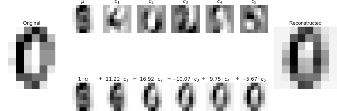
Reconstruct data
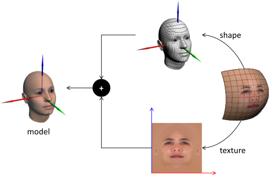
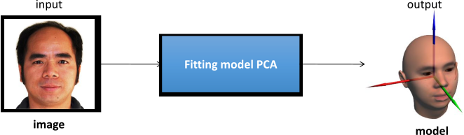
3D Head Model
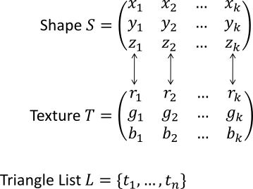
Fitting 3D Head Model
9.6 Linear Discriminant Analysis
Introduction
Linear Discriminant Analysis (LDA) is a supervised dimension-reduction tool that the goal is to find the feature subspace that optimizes class separability.
Algorithm
Input: Data \mathcal{D}=\{(\boldsymbol{x}_{1},y_{1}),...,(\boldsymbol{x}_{n},y_{n})\},\boldsymbol{x}_{i}\in\mathbb{R}^{D},y_{i}\in\{c_{1},...,c_{k}\}
Output: projection matrix W
For each class, compute the D dimensional mean vector.
Construct the between-class scatter matrix S_{B} and the within-class scatter matrix S_{W}.
Compute the eigenvectors and corresponding eigenvalues of the matrix S_{W}^{-1}S_{B}.
Sort the eigenvalues by decreasing order to rank the corresponding eigenvectors.
Choose the k eigenvectors that correspond to the k largest eigenvalues to construct a D\times D-dimensional transformation matrix W; the eigenvectors are the columns of this matrix.
- Transform the D-dimensional input dataset \mathcal{D} using the projection matrix W to obtain the new k-dimensional feature subspace.