10 MIXTURE MODELS
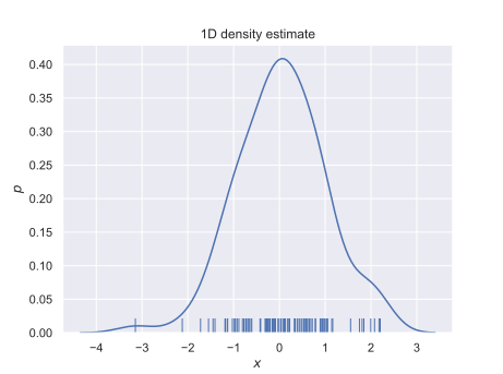
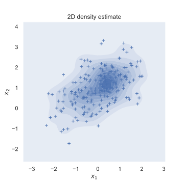
Unsupervised Problem
- Given data set \mathcal{D}=\{\boldsymbol{x}_{1},...,\boldsymbol{x}_{n}\}, find its distribution p(\boldsymbol{x}\mid\mathcal{D})
10.1 Introduction
Gaussian Distribution
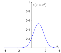
Univariate Normal Distribution
- A random variable X is normally distributed with parameters ({\color{red}\mu},{\color{red}\sigma}^{{\color{red}2}}), denoted as \mathcal{N}(x;{\color{red}\mu},{\color{red}\sigma}^{{\color{red}2}}) if its density function is given by \begin{equation} p(x;{\color{red}\mu},{\color{red}\sigma}^{{\color{red}2}})=\mathcal{N}(x;{\color{red}\mu},{\color{red}\sigma}^{{\color{red}2}})=\frac{1}{\sqrt{2\pi{\color{red}\sigma}^{{\color{red}2}}}}\exp\left(-\frac{(x-{\color{red}\mu})^{2}}{2{\color{red}\sigma}^{{\color{red}2}}}\right) \end{equation}
Multivariate Normal Distribution
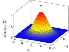
A multivariate normal distribution is defined by two parameters:
mean vector {\color{red}\boldsymbol{\mu}}\in\mathbb{R}^{D}
covariance matrix {\color{red}\Sigma}\in\mathbb{R}^{D\times D}, where {\color{red}\Sigma} is a positive definite matrix.
The density function is given by \begin{equation} p(\boldsymbol{x};{\color{red}\boldsymbol{\mu}},{\color{red}\Sigma})=\mathcal{N}(\boldsymbol{x};{\color{red}\boldsymbol{\mu}},{\color{red}\Sigma})=\dfrac{1}{(2\pi)^{\frac{D}{2}}|{\color{red}\Sigma}|^{\frac{1}{2}}}\exp\left[-\dfrac{1}{2}(\boldsymbol{x}-\boldsymbol{{\color{red}\mu}})^{T}{\color{red}\Sigma}^{-1}(\boldsymbol{x}-{\color{red}\boldsymbol{\mu}})\right] \end{equation}
A random vector-valued variable \boldsymbol{x}=(x_{1},x_{2},...,x_{D}) is called normally distributed if all linear combinations of its components x_{i},i=1,...,D is normally distributed.
In other words: \exists{\color{red}\mu}\in\mathbb{R},{\color{red}\sigma}\in\mathbb{R}:\boldsymbol{w}\cdot\boldsymbol{x}^{\intercal}\sim\mathcal{N}({\color{red}\mu},{\color{red}\sigma}^{2}),\forall w\in\mathbb{R}^{D}.
A square matrix A n\times n is called positive definite if \boldsymbol{z}^{\intercal}A\boldsymbol{z}>0,\forall\boldsymbol{z}\in\mathbb{R}^{n},\boldsymbol{z}\neq\boldsymbol{0}.
Gaussian Model
What is a Gaussian Model?
Input data set \mathcal{D}=\{\boldsymbol{x}_{1},...,\boldsymbol{x}_{n}\}
The likelihood of \boldsymbol{x} given a Gaussian model is p(\boldsymbol{x}\mid\boldsymbol{\mu},\Sigma)=\dfrac{1}{(2\pi)^{\frac{D}{2}}|\Sigma|^{\frac{1}{2}}}\exp\left[-\dfrac{1}{2}(\boldsymbol{x}-\boldsymbol{\mu})^{T}\Sigma^{-1}(\boldsymbol{x}-\boldsymbol{\mu})\right] where D is the dimension of \boldsymbol{x}, \boldsymbol{\mu} is the mean and \Sigma is the covariance matrix of the Gaussian. \Sigma is often diagonal.
Objective: maximize the likelihood p(\mathcal{D}\mid\boldsymbol{\mu},\Sigma) of the data \mathcal{D} drawn from the Gaussian model \begin{equation} \arg\max_{\boldsymbol{\mu},\Sigma}p(\mathcal{D}\mid\boldsymbol{\mu},\Sigma)=\arg\max_{\boldsymbol{\mu},\Sigma}\prod_{i=1}^{n}p(\boldsymbol{x}_{i}\mid\boldsymbol{\mu},\Sigma) \end{equation}
Closed-form Solution
- Solve the optimization problem (1), we have \begin{equation} \hat{\boldsymbol{\mu}}=\frac{1}{n}\sum_{i=1}^{n}\boldsymbol{x}_{i} \end{equation} \begin{equation} \hat{\Sigma}=\frac{1}{n-1}\sum_{i=1}^{n}(\boldsymbol{x}_{i}-\hat{\boldsymbol{\mu}})(\boldsymbol{x}_{i}-\hat{\boldsymbol{\mu}})^{\intercal} \end{equation}
Gaussian Mixture Model
What is a Gaussian Mixture Model?
A Gaussian Mixture Model (GMM) is a distribution
The likelihood given a Gaussian distribution is \begin{equation} \mathcal{N}(\boldsymbol{x}\mid\boldsymbol{\mu},\Sigma)=\dfrac{1}{(2\pi)^{\frac{D}{2}}|\Sigma|^{\frac{1}{2}}}\exp\left[-\dfrac{1}{2}(\boldsymbol{x}-\boldsymbol{\mu})^{T}\Sigma^{-1}(\boldsymbol{x}-\boldsymbol{\mu})\right] \end{equation} where D is the dimension of \boldsymbol{x}, \boldsymbol{\mu} is the mean and \Sigma is the covariance matrix of the Gaussian. \Sigma is often diagonal.
The likelihood given a GMM is \begin{equation} p(\boldsymbol{x})=\sum_{k=1}^{K}w_{k}\cdot\mathcal{N}(\boldsymbol{x}\mid\boldsymbol{\mu}_{k},\Sigma_{k}) \end{equation} where K is the number of Gaussians and w_{k} is the weight of Gaussian k, with \begin{equation} \sum_{k=1}^{K}w_{k}=1\text{ and }w_{k}\geq0 \end{equation}
Characteristics of a GMM
ANNs are universal approximators of functions
GMMs are universal approximators of densities (as long as there are enough Gaussians of course)
Even diagonal GMMs are universal approximators.
Full rank GMMs are not easy to handle: number of parameters is the square of the number of dimensions.
GMMs can be trained by maximum likelihood using an efficient algorithm: Expectation-Maximization.
Applications
Practical Applications using GMMs
Biometric person authentication (using voice, face, handwriting, etc):
one GMM for the client
one GMM for all the others
Bayes decision \Longrightarrow likelihood ratio
Any highly imbalanced classification task
one GMM per class, tuned by maximum likelihood
Bayes decision \Longrightarrow likelihood ratio
Dimensionality reduction
Quantization
10.2 The EM Algorithm
Introduction
Basics of Expectation-Maximization
Objective: maximize the likelihood p(\mathcal{D}\mid\theta) of the data \mathcal{D}=\{\boldsymbol{x}_{1},...,\boldsymbol{x}_{n}\} drawn from an unknown distribution, given the model parameterized by \theta: \begin{equation} \theta^{\ast}=\arg\max_{\theta}p(\mathcal{D}\mid\theta)=\arg\max_{\theta}\prod_{i=1}^{n}p(\boldsymbol{x}_{i}\mid\theta) \end{equation}
Basic ideas of EM:
- Introduce a hidden variable such that its knowledge would simplify the maximization of p(\mathcal{D}\mid\theta)
At each iteration of the algorithm:
E-Step: estimate the distribution of the hidden variable given the data and the current value of the parameters
M-Step: modify the parameters in order to maximize the joint distribution of the data and the hidden variable
Graphical Interpretation
EM for GMM - Graphical View
Hidden variable: for each point, which Gaussian generated it?
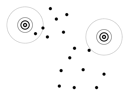
E-Step: for each point, estimate the probability that each Gaussian generated it
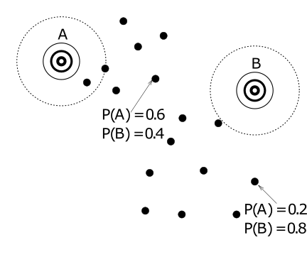
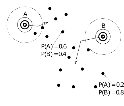
M-Step: modify the parameters according to the hidden variable to maximize the likelihood of the data (and the hidden variable)
More Formally
EM: More Formally
Let us call the hidden variable Q and consider the following auxiliary function: \begin{equation} A(\theta,\theta^{t})=\mathbb{E}_{Q}\left[\log p(\mathcal{D},Q\mid\theta)\mid\mathcal{D},\theta^{t}\right] \end{equation}
It can be shown that maximizing A \begin{equation} \theta^{t+1}=\arg\max_{\theta}A(\theta,\theta^{t}) \end{equation} always increases the likelihood of the data p(\mathcal{D}\mid\theta^{t+1}), and a maximum of A corresponds to a maximum of the likelihood.
Proof of Convergence
First let us develop the auxiliary function: \begin{align} A(\theta,\theta^{t}) & =\mathbb{E}_{Q}\left[\log p(\mathcal{D},Q\mid\theta)\mid\mathcal{D},\theta^{t}\right]\\ & =\sum_{q\in Q}P(q\mid\mathcal{D},\theta^{t})\log p(\mathcal{D},q\mid\theta)\nonumber \\ & =\sum_{q\in Q}P(q\mid\mathcal{D},\theta^{t})\log\left(P(q\mid\mathcal{D},\theta)\cdot p(\mathcal{D}\mid\theta)\right)\nonumber \\ & =\left[\sum_{q\in Q}P(q\mid\mathcal{D},\theta^{t})\log P(q\mid\mathcal{D},\theta)\right]+\log p(\mathcal{D}\mid\theta)\nonumber \end{align}
then if we evaluate it at \theta^{t} \begin{equation} A(\theta^{t},\theta^{t})=\left[\sum_{q\in Q}P(q\mid\mathcal{D},\theta^{t})\log P(q\mid\mathcal{D},\theta^{t})\right]+\log p(\mathcal{D}\mid\theta^{t}) \end{equation}
the difference between two consecutive log likelihoods of the data can be written as \log p(\mathcal{D}\mid\theta)-\log p(\mathcal{D}\mid\theta^{t})= \begin{equation} A(\theta,\theta^{t})-A(\theta^{t},\theta^{t})+\left[\sum_{q\in Q}P(q\mid\mathcal{D},\theta^{t})\log\dfrac{P(q\mid\mathcal{D},\theta^{t})}{P(q\mid\mathcal{D},\theta)}\right] \end{equation}
Hence,
since the last part of the equation is a Kullback-Leibler divergence which is always positive or null,
if A increases, the log likelihood of the data also increases
Moreover, one can show that when A is maximum, the likelihood of the data is also at a maximum.
10.3 EM for Coins
A coin experiment
Estimate the bias of two coins:
Chosen one of the two coins at random.
Flipped that same coin 10 times.
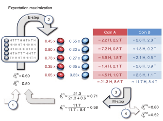
How can you provide a reasonable estimate of each coin bias? Let’s refer to these coins as coin A and coin B and their bias as \theta_{A} and \theta_{B}.
We see which coin is flipped
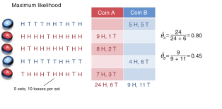
We don’t see which coin is flipped
Using EM algorithm
EM starts with an initial guess of the parameters.
In the E-step, a probability distribution over possible completions is computed using the current parameters. The counts shown in the table are the expected numbers of heads and tails according to this distribution.
In the M-step, new parameters are determined using the current completions.
After several repetitions of the E-step and M-step, the algorithm converges.
We don’t see which coin is flipped (cont.)
| Loop | \theta_{A} | \theta_{B} |
|---|---|---|
| 0 | 0.60 | 0.50 |
| 1 | 0.71 | 0.58 |
| 2 | 0.75 | 0.57 |
| 3 | 0.77 | 0.55 |
| 4 | 0.78 | 0.53 |
| 5 | 0.79 | 0.53 |
| 6 | 0.79 | 0.52 |
| 7 | 0.80 | 0.52 |
| 8 | 0.80 | 0.52 |
| 9 | 0.80 | 0.52 |
| 10 | 0.80 | 0.52 |
10.4 EM for GMMs
Auxiliary Function
EM for GMM: Auxiliary Function
We can now write the joint likelihood of all the \mathcal{D} and q: \begin{equation} p(\mathcal{D},Q\mid\boldsymbol{\theta})=\prod_{i=1}^{n}\prod_{k=1}^{K}P(k\mid\boldsymbol{\theta})^{q_{i,k}}p(x_{i}\mid k,\boldsymbol{\theta})^{q_{i,k}} \end{equation}
which in log gives \begin{equation} \log p(\mathcal{D},Q\mid\boldsymbol{\theta})=\sum_{i=1}^{n}\sum_{k=1}^{K}q_{i,k}\log P(k\mid\boldsymbol{\theta})+q_{i,k}\log p(x_{i}\mid k,\boldsymbol{\theta}) \end{equation}
Let us now write the corresponding auxiliary function: \begin{align} A(\boldsymbol{\theta},\boldsymbol{\theta}^{t}) & =\mathbb{E}_{Q}\left[\log p(\mathcal{D},Q\mid\boldsymbol{\theta})\mid\mathcal{D},\boldsymbol{\theta}^{t}\right]\\ & =\mathbb{E}_{Q}\left[\sum_{i=1}^{n}\sum_{k=1}^{K}q_{i,k}\log P(k\mid\boldsymbol{\theta})+q_{i,k}\log p(x_{i}\mid k,\boldsymbol{\theta})\mid\mathcal{D},\boldsymbol{\theta}^{t}\right]\nonumber \\ & =\sum_{i=1}^{n}\sum_{k=1}^{K}\mathbb{E}_{Q}[q_{i,k}\mid\mathcal{D},\boldsymbol{\theta}^{t}]\log P(k\mid\boldsymbol{\theta})+\mathbb{E}_{Q}[q_{i,k}\mid\mathcal{D},\boldsymbol{\theta}^{t}]\log p(x_{i}\mid k,\boldsymbol{\theta})\nonumber \end{align}
E-Step
E-Step
- Hence, the E-Step estimates the posterior: \begin{align} \mathbb{E}_{Q}[q_{i,k}\mid\mathcal{D},\boldsymbol{\theta}^{t}] & =1\cdot P(q_{i,k}=1\mid\mathcal{D},\boldsymbol{\theta}^{t})+0\cdot P(q_{i,k}=0\mid\mathcal{D},\boldsymbol{\theta}^{t})\\ & =P(k\mid x_{i},\boldsymbol{\theta}^{t})=\dfrac{p(x_{i}\mid k,\boldsymbol{\theta}^{t})P(k\mid\boldsymbol{\theta}^{t})}{p(x_{i}\mid\boldsymbol{\theta}^{t})}\nonumber \end{align}
M-Step
M-Step
M-step finds the parameters \boldsymbol{\theta}=\left\{ \mu,\sigma^{2},w\right\} that maximizes A, hence searching for \frac{\partial A}{\partial\theta}=0 for each parameter (means \mu_{k}, variances \sigma_{k}^{2}, and weights w_{k}).
Note however that \left\{ w_{k}\right\} _{k=1}^{K} should sum to 1.
M-Step for Means
\begin{equation} A(\boldsymbol{\theta},\boldsymbol{\theta}^{t})=\sum_{i=1}^{n}\sum_{k=1}^{K}\mathbb{E}_{Q}[q_{i,k}\mid\mathcal{D},\boldsymbol{\theta}^{t}]\log P(k\mid\boldsymbol{\theta})+\mathbb{E}_{Q}[q_{i,k}\mid\mathcal{D},\boldsymbol{\theta}^{t}]\log p(x_{i}\mid k,\boldsymbol{\theta}) \end{equation}
\begin{align*} \frac{\partial A}{\partial\mu_{k}} & =\sum_{i=1}^{n}\frac{\partial A}{\partial\log p(x_{i}\mid k,\theta)}\frac{\partial\log p(x_{i}\mid k,\theta)}{\partial\mu_{k}}\\ & =\sum_{i=1}^{n}P(k\mid x_{i},\theta^{t})\frac{\partial\log p(x_{i}\mid k,\theta)}{\partial\mu_{k}}\\ & =\sum_{i=1}^{n}P(k\mid x_{i},\theta^{t})\frac{(x_{i}-\mu_{k})}{\sigma_{k}^{2}}=0 \end{align*}
- removing constant terms in the sum \sum_{i=1}^{n}P(k\mid x_{i},\theta^{t})x_{i}-\sum_{i=1}^{n}P(k\mid x_{i},\theta^{t})\mu_{k}=0 \hat{\mu}_{k}=\dfrac{\sum_{i=1}^{n}P(k\mid x_{i},\theta^{t})x_{i}}{\sum_{i=1}^{n}P(k\mid x_{i},\theta^{t})}
M-Step for Variances
A(\boldsymbol{\theta},\boldsymbol{\theta}^{t})=\sum_{i=1}^{n}\sum_{k=1}^{K}\mathbb{E}_{Q}[q_{i,k}\mid\mathcal{D},\boldsymbol{\theta}^{t}]\log P(k\mid\boldsymbol{\theta})+\mathbb{E}_{Q}[q_{i,k}\mid\mathcal{D},\boldsymbol{\theta}^{t}]\log p(x_{i}\mid k,\boldsymbol{\theta}) \begin{align*} \frac{\partial A}{\partial\sigma_{k}^{2}} & =\sum_{i=1}^{n}\frac{\partial A}{\partial\log p(x_{i}\mid k,\theta)}\frac{\partial\log p(x_{i}\mid k,\theta)}{\partial\sigma_{k}^{2}}\\ & =\sum_{i=1}^{n}P(k\mid x_{i},\theta^{t})\frac{\partial\log p(x_{i}\mid k,\theta)}{\partial\sigma_{k}^{2}}\\ & =\sum_{i=1}^{n}P(k\mid x_{i},\theta^{t})\left(\frac{(x_{i}-\mu_{k})^{2}}{2\sigma_{k}^{4}}-\frac{1}{2\sigma_{k}^{2}}\right)=0 \end{align*} \hat{\sigma}_{k}^{2}=\dfrac{\sum_{i=1}^{n}P(k\mid x_{i},\theta^{t})(x_{i}-\hat{\mu}_{k})^{2}}{\sum_{i=1}^{n}P(k\mid x_{i},\theta^{t})}
M-Step for Weights
We have the constraint that all weights w_{k} should be positive and sum to 1: \sum_{k=1}^{K}w_{k}=1
Incorporating it into the system: J(\theta,\theta^{t})=A(\theta,\theta^{t})+\left(1-\sum_{k=1}^{K}w_{k}\right)\lambda_{k} where \lambda_{k} are Lagrange multipliers.
So we need to derive J with respect to w_{k} and to set it to 0. \begin{align*} \frac{\partial J}{\partial w_{k}} & =\frac{\partial J}{\partial A(\theta,\theta^{t})}\frac{\partial A(\theta,\theta^{t})}{\partial w_{k}}-\lambda_{k}\\ & =1\cdot\left(\sum_{i=1}^{n}P(k\mid x_{i},\theta^{t})\cdot\frac{1}{w_{k}}\right)-\lambda_{k}=0 \end{align*} \hat{w}_{k}=\dfrac{\sum_{i=1}^{n}P(k\mid x_{i},\theta^{t})}{\lambda_{k}}
and incorporating the probabilistic constraint, we get \hat{w}_{k}=\dfrac{\sum_{i=1}^{n}P(k\mid x_{i},\theta^{t})}{\sum_{j=1}^{K}\sum_{i=1}^{n}P(j\mid x_{i},\theta^{t})}=\frac{1}{n}\sum_{i=1}^{n}P(k\mid x_{i},\theta^{t})
Update Rules
\begin{equation} \begin{array}{lll} \text{Means} & & \hat{\mu}_{k}=\dfrac{\sum_{i=1}^{n}P(k\mid x_{i},\theta^{t})x_{i}}{\sum_{i=1}^{n}P(k\mid x_{i},\theta^{t})}\\ \text{Variances} & & \hat{\sigma}_{k}^{2}=\dfrac{\sum_{i=1}^{n}P(k\mid x_{i},\theta^{t})(x_{i}-\hat{\mu}_{k})^{2}}{\sum_{i=1}^{n}P(k\mid x_{i},\theta^{t})}\\ \text{Weights} & & \hat{w}_{k}=\dfrac{1}{n}\sum_{i=1}^{n}P(k\mid x_{i},\theta^{t}) \end{array} \end{equation}
Example
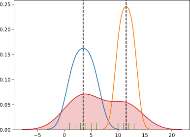
- Data \mathcal{D}=\{1,2,3,4,5,6,10,11,12,13\} generated by two Gaussians \mathcal{N}(\mu_{1},\sigma_{1}) and \mathcal{N}(\mu_{2},\sigma_{2})
Example
Estimate the most likely Gaussians \mathcal{N}(\mu_{1},\sigma_{1}) and \mathcal{N}(\mu_{2},\sigma_{2}) from \mathcal{D}
Loop \mu_{1} \sigma_{1} \mu_{2} \sigma_{2} 0 2 1 11 1 1 3.495413364585706 1.7060277624010254 11.48493211841284 1.152919810380393 2 3.5012090905616713 1.710016971284593 11.500336746451783 1.1180916981781446 3 3.5013264210256705 1.7102090502730485 11.500411717617954 1.1179889840886608 4 3.5013290606968535 1.7102137326222728 11.500412673611843 1.1179885261658662 5 3.5013291208365427 1.7102138400004387 11.50041269402295 1.1179885191522907 6 3.501329122208362 1.7102138424510698 11.500412694486043 1.1179885189985401 7 3.5013291222396563 1.710213842506978 11.500412694496601 1.1179885189950438 8 3.5013291222403704 1.7102138425082534 11.500412694496841 1.1179885189949643 9 3.501329122240387 1.7102138425082827 11.500412694496847 1.1179885189949623 10 3.501329122240387 1.7102138425082831 11.500412694496848 1.1179885189949623 11 3.501329122240387 1.7102138425082831 11.500412694496848 1.1179885189949623
10.5 Practical Issues
Initialization
Initialization
EM is an iterative procedure that is very sensitive to initial conditions!
Start from trash \to end up with trash.
Hence, we need a good and fast initialization procedure.
Often used: K-Means.
Other options: hierarchical K-Means, Gaussian splitting.
Capacity Control
Capacity Control
How to control the capacity with GMMs?
selecting the number of Gaussians
constraining the value of the variances to be far from 0 (small variances \Longrightarrow large capacity)
Use cross-validation on the desired criterion (Maximum Likelihood, classification...)
Adaptation
Adaptation Techniques
In some cases, you have access to only a few examples coming from the target distribution...
... but many coming from a nearby distribution!
How can we profit from the big nearby dataset?
Solution: use adaptation techniques.
The most well known and used for GMMs: the Maximum A Posteriori adaptation.
MAP Adaptation
Normal maximum likelihood training for a dataset \mathcal{D}: \begin{equation} \theta^{\ast}=\arg\max_{\theta}p(\mathcal{D}\mid\theta) \end{equation}
Maximum A Posteriori (MAP) training: \begin{align} \theta^{\ast} & =\arg\max_{\theta}p(\theta\mid\mathcal{D})\\ & =\arg\max_{\theta}\frac{p(\mathcal{D}\mid\theta)p(\theta)}{p(\mathcal{D})}\nonumber \\ & =\arg\max_{\theta}p(\mathcal{D}\mid\theta)p(\theta)\nonumber \end{align} where p(\theta) represents your prior belief about the distribution of the parameters \theta.
Implementation
Which kind of prior distribution for p(\theta)?
Two objectives:
constraining \theta to reasonable values
keep the EM algorithm tractable
Use conjugate priors:
Dirichlet distribution for weights
Gaussian densities for means and variances
What is a Conjugate Prior?
A conjugate prior is chosen such that the corresponding posterior belongs to the same functional family as the prior.
So we would like that p(X\mid\theta)p(\theta) is distributed according to the same family as p(\theta) and tractable.
Example
Likelihood is Gaussian p(X\mid\theta)=K_{1}\exp\left(-\frac{(x_{1}-\mu_{1})^{2}}{2\sigma_{1}^{2}}\right)
Prior is Gaussian p(\theta)=K_{2}\exp\left(-\frac{(x_{2}-\mu_{2})^{2}}{2\sigma_{2}^{2}}\right)
Posterior is Gaussian \begin{array}{lll} p(X\mid\theta)p(\theta) & = & K_{1}K_{2}\exp\left(-\dfrac{(x_{1}-\mu_{1})^{2}}{2\sigma_{1}^{2}}-\dfrac{(x_{2}-\mu_{2})^{2}}{2\sigma_{2}^{2}}\right)\\ & = & K_{3}\exp\left(-\dfrac{(x-\mu)^{2}}{2\sigma^{2}}\right) \end{array}
Conjugate Prior of Multinomials
Multinomial distribution: \begin{equation} p(X_{1}=x_{1},...,X_{K}=x_{K}\mid\theta)=\dbinom{n}{x_{1}\cdots x_{K}}\prod\limits_{k=1}^{K}\theta_{k}^{x_{k}} \end{equation} where x_{k} are nonnegative integers and \sum_{k=1}^{K}x_{k}=n
Dirichlet distribution with parameter u: \begin{equation} P(\theta\mid u)=\frac{1}{Z(u)}\prod\limits_{k=1}^{K}\theta_{k}^{u_{k}-1} \end{equation} where \theta_{1},...,\theta_{K}\geq0 and \sum_{k=1}^{K}\theta_{k}=1 and u_{1},...,u_{K}\geq0
Conjugate prior = dirichlet with parameter x+u: \begin{equation} P(X,\theta\mid u)=\frac{1}{Z}\prod\limits_{k=1}^{K}\theta_{k}^{x_{k}+u_{k}-1} \end{equation}
Examples of Conjugate Priors
| likelihood p(\mathcal{D}\mid\theta) | conjugate prior p(\theta) | posterior p(\theta\mid\mathcal{D}) |
|---|---|---|
| Gaussian | Gaussian | Gaussian |
| Binomial | Beta | Beta |
| Poisson | Gamma | Gamma |
| Multinomial | Dirichlet | Dirichlet |
Simple Implementation for MAP-GMMs
Simple Implementation
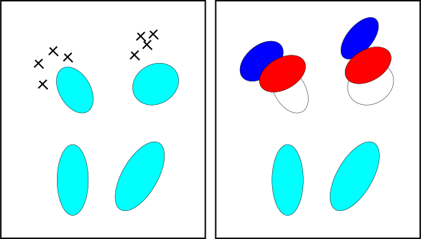
Train a generic prior model p with large amount of available data \Longrightarrow\left\{ w_{k}^{p},\mu_{k}^{p},\sigma_{k}^{p}\right\}
One hyper-parameter: \alpha\in[0,1]: faith on prior model
Weights: \hat{w}_{k}=\left[\alpha w_{k}^{p}+(1-\alpha)\sum_{i=1}^{n}P(k\mid x_{i})\right]\gamma where \gamma is a normalization factor (so that \sum_{k}w_{k}=1)
Means: \hat{\mu}_{k}=\alpha\mu_{k}^{p}+(1-\alpha)\frac{\sum_{i=1}^{n}P(k\mid x_{i})x_{i}}{\sum_{i=1}^{n}P(k\mid x_{i})}
Variances: \hat{\sigma}_{k}=\alpha(\sigma_{k}^{p}+\mu_{k}^{p}\mu_{k}^{p})+(1-\alpha)\frac{\sum_{i=1}^{n}P(k\mid x_{i})x_{i}x_{i}}{\sum_{i=1}^{n}P(k\mid x_{i})}-\mu_{k}^{p}\mu_{k}^{p}
Adapted GMMs for Person Authentication
Person authentication task: \text{accept access if }P(S_{i}\mid\mathcal{D})>P(\bar{S}_{i}\mid\mathcal{D}) with S_{i} a client, \bar{S}_{i} all the other persons, and \mathcal{D} an access attributed to S_{i}.
Using Bayes theorem, this becomes: \frac{P(\mathcal{D}\mid S_{i})}{P(\mathcal{D}\mid\bar{S}_{i})}>\frac{P(\bar{S}_{i})}{P(S_{i})}=\Delta_{S_{i}}\approx\Delta
P(\mathcal{D}\mid\bar{S}_{i}) is trained on a large dataset.
P(\mathcal{D}\mid S_{i}) is MAP adapted from P(\mathcal{D}\mid\bar{S}_{i}).
\Delta is found on a separate validation set to optimize a given criterion.