17 ATTENTION MECHANISMS
17.1 Attention Functions
What is Attention?
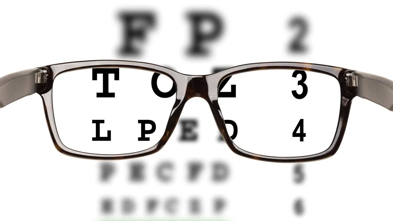
Attention is, to some extent, motivated by how we pay visual attention to different regions of an image or correlate words in one sentence.
Attention Functions
Attention Function
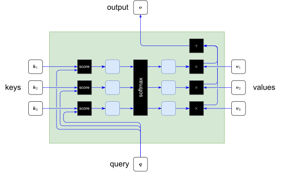
An attention function can be described as mapping a query \boldsymbol{q} and a set of key-value pairs \{(\boldsymbol{k}_{i},\boldsymbol{v}_{i})\} to an output \boldsymbol{o}
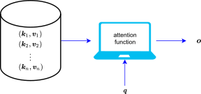
The output is computed as a weighted sum of the values, where the weight assigned to each value is computed by a compatibility function \alpha of the query with the corresponding key. \begin{equation} \boldsymbol{o}=\text{Attention}(\boldsymbol{q},\boldsymbol{k}_{1...n},\boldsymbol{v}_{1...n})=\sum_{i=1}^{n}\alpha(\boldsymbol{q},\boldsymbol{k}_{i})\boldsymbol{v}_{i} \end{equation} where \sum_{i=1}^{n}\alpha(\boldsymbol{q},\boldsymbol{k}_{i})=1
Type of attention
Type of attention
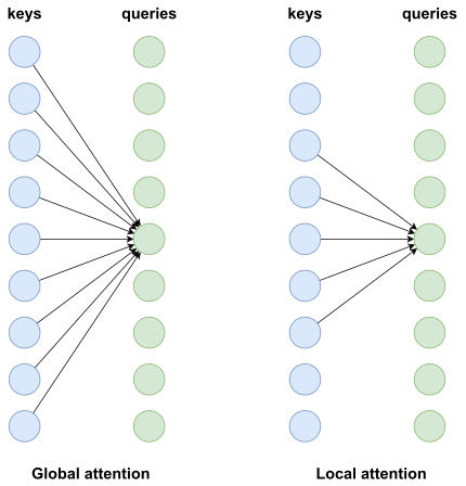
In global attention, we consider all the keys.
In local attention, we consider only a subset of the keys.
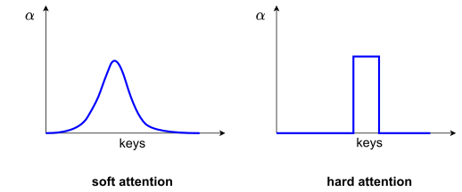
In soft attention, the function \alpha varies smoothly over its domain and, as a result, it is differentiable.
In hard attention, the function \alpha determine whether to attend to a region or not, which means that the function has many abrupt changes over its domain.
17.2 Attention Pooling
NonParametric Kernel Regression
Kernel Regression
Problem: Given a dataset of input-output pairs \mathcal{D}=\{(\boldsymbol{x}_{1},y_{1}),\ldots,(\boldsymbol{x}_{N},y_{N})\}, how to learn f to predict the output \hat{y}=f(\boldsymbol{x}) for any new input \boldsymbol{x}?
Solution: Consider (\boldsymbol{x}_{i},y_{i}) as a pair of key-value and x as query
key value \boldsymbol{x}_{1} y_{1} \vdots \vdots \boldsymbol{x}_{N} y_{N}
\begin{equation} \hat{y}=\sum_{i=1}^{N}\alpha(\boldsymbol{x},\boldsymbol{x}_{i})y_{i}, \end{equation}
- We define \alpha using a Gaussian kernel \begin{equation} \alpha(\boldsymbol{x},\boldsymbol{x}_{i})=\frac{\exp\left[-\frac{1}{2}\left\Vert \boldsymbol{x}-\boldsymbol{x}_{i}\right\Vert ^{2}\right]}{\sum_{j=1}^{n}\exp\left[-\frac{1}{2}\left\Vert \boldsymbol{x}-\boldsymbol{x}_{j}\right\Vert ^{2}\right]}. \end{equation} and plug it into equation (17)
\begin{equation} \begin{split}\begin{aligned}\hat{y} & =\sum_{i=1}^{N}\alpha(\boldsymbol{x},\boldsymbol{x}_{i})y_{i}\\ & =\sum_{i=1}^{N}\frac{\exp\left[-\frac{1}{2}\left\Vert \boldsymbol{x}-\boldsymbol{x}_{i}\right\Vert ^{2}\right]}{\sum_{j=1}^{N}\exp\left[-\frac{1}{2}\left\Vert \boldsymbol{x}-\boldsymbol{x}_{j}\right\Vert ^{2}\right]}y_{i} \end{aligned} \end{split} \end{equation}
- A key \boldsymbol{x}_{i} that is closer to the given query \boldsymbol{x} will get more attention via a larger attention weight assigned to the key’s corresponding value y_{i}.
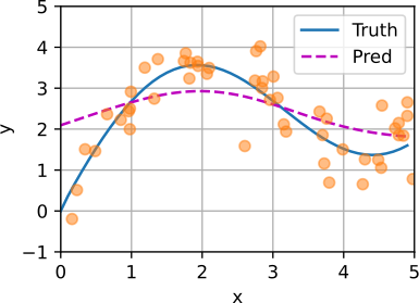
Example 1
Generate an artificial dataset including 50 training examples and 50 testing examples according to the following nonlinear function with the noise term \epsilon\sim\mathcal{N}(0,0.5) y=2\sin(x)+x^{0.8}+\epsilon
Find the kernel regression
Parametric Kernel Regression
Parametric Kernel Regression
Kernel regression enjoys the consistency benefit: given enough data this model converges to the optimal solution.
Nonetheless, we can easily integrate learnable parameters.
In the following the distance between the query \boldsymbol{x} and the key \boldsymbol{x}_{i} is multiplied a learnable parameter {\color{red}w}:
\begin{equation} \begin{split}\begin{aligned}\hat{y} & =\sum_{i=1}^{N}\frac{\exp\left[-\frac{1}{2}\left(\left\Vert \boldsymbol{x}-\boldsymbol{x}_{i}\right\Vert {\color{red}w}\right)^{2}\right]}{\sum_{j=1}^{N}\exp\left[-\frac{1}{2}\left(\left\Vert \boldsymbol{x}-\boldsymbol{x}_{j}\right\Vert {\color{red}w}\right)^{2}\right]}y_{i}\end{aligned} \end{split} \end{equation}
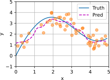
Example 2
Generate an artificial dataset including 50 training examples and 50 testing examples according to the following nonlinear function with the noise term \epsilon\sim\mathcal{N}(0,0.5) y=2\sin(x)+x^{0.8}+\epsilon
Find the parametric kernel regression
17.3 Attention Scoring Functions
Introduction
- We use an attention scoring function and softmax function to compute the attention function
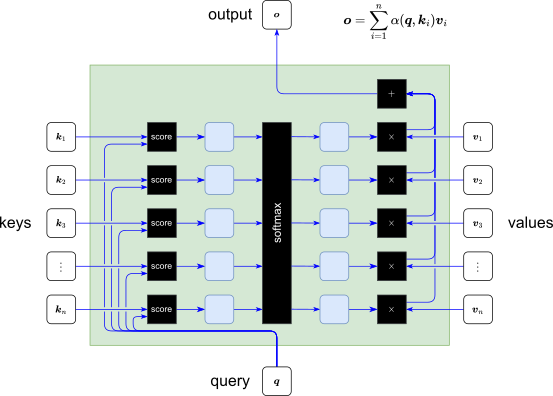
An attention scoring function is used to measure the relevance between a query and a key

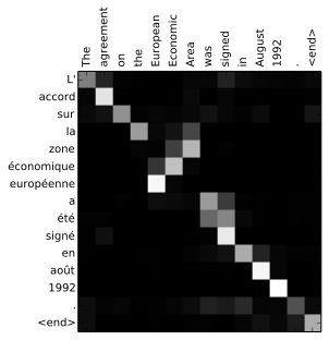
Attention scores from different sources
English: “The agreement on the European Economic Area was signed in August 1992”
French: “L’accord sur la zone économique européenne a été signé en août 1992.”
Some Attention Scoring Functions
Additive score (Bahdanau et al. 2015) \begin{equation} \text{score}(\boldsymbol{q},\boldsymbol{k})={\color{red}\boldsymbol{w}}_{v}^{\top}\text{tanh}({\color{red}W}_{q}\boldsymbol{q}+{\color{red}W}_{k}\boldsymbol{k}) \end{equation}
Multiplicative score (Luong et al. 2015) \begin{equation} \text{score}(\boldsymbol{q},\boldsymbol{k})=\boldsymbol{q}^{\top}{\color{red}W}\boldsymbol{k} \end{equation}
Dot-product score (Luong et al. 2015) \begin{equation} \text{score}(\boldsymbol{q},\boldsymbol{k})=\boldsymbol{q}^{\top}\boldsymbol{k} \end{equation}
Scaled dot-product score (Vaswani et al. 2017) \begin{equation} \text{score}(\boldsymbol{q},\boldsymbol{k})=\frac{\boldsymbol{q}^{\top}\boldsymbol{k}}{\sqrt{dim(\boldsymbol{k})}} \end{equation}
Cosine score (Graves et al. 2014)
\begin{equation} \text{score}(\boldsymbol{q},\boldsymbol{k})=\text{cosine}(\boldsymbol{q},\boldsymbol{k}) \end{equation}
Example 1
- Using dot-product score to calculate the output \boldsymbol{o} given that
\boldsymbol{q}=\left(\begin{array}{c} 1\\ -1\\ 2 \end{array}\right),\boldsymbol{k}_{1}=\left(\begin{array}{c} 2\\ 1\\ -2 \end{array}\right),\boldsymbol{v}_{1}=\left(\begin{array}{c} 2\\ 3 \end{array}\right),\boldsymbol{k}_{2}=\left(\begin{array}{c} 1\\ 2\\ -1 \end{array}\right),\boldsymbol{v}_{2}=\left(\begin{array}{c} 1\\ 2 \end{array}\right),\boldsymbol{k}_{3}=\left(\begin{array}{c} 3\\ -2\\ 0 \end{array}\right),\boldsymbol{v}_{3}=\left(\begin{array}{c} 3\\ 1 \end{array}\right)
17.4 Attention Layer
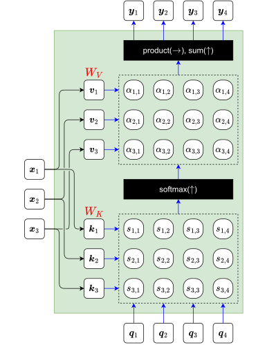
Attention Layer
Input:
Query vectors: Q
Memory vectors: X
Output:
- Output vectors: Y
Parameters: {\color{red}W_{K}},{\color{red}W_{V}}
Function:
Y=\text{AttentionLayer}(X,Q;{\color{red}W_{K}},{\color{red}W_{V}})
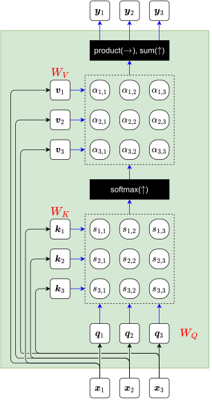
Self-Attention Layer
Input:
- Input vectors: X
Output:
- Output vectors: Y
Parameters: {\color{red}W_{K}},{\color{red}W_{V}},{\color{red}W_{Q}}
Function:
Y=\text{SelfAttentionLayer}(X;{\color{red}W_{K}},{\color{red}W_{V}},{\color{red}W_{Q}})
Example 2
- Calculate the output of the self-attention layer given that X=\left(\begin{array}{ccc} \boldsymbol{x}_{1} & \boldsymbol{x}_{2} & \boldsymbol{x}_{3}\end{array}\right)=\left(\begin{array}{ccc} 1 & 0 & 1\\ 0 & 2 & 1\\ 1 & 0 & 1\\ 0 & 2 & 1 \end{array}\right)
{\color{red}W_{K}}=\left(\begin{array}{cccc} 0 & 1 & 0 & 1\\ 0 & 1 & 1 & 1\\ 1 & 0 & 0 & 0 \end{array}\right),{\color{red}W_{Q}}=\left(\begin{array}{cccc} 1 & 1 & 0 & 0\\ 0 & 0 & 0 & 1\\ 1 & 0 & 1 & 1 \end{array}\right),{\color{red}W_{V}}=\left(\begin{array}{cccc} 0 & 0 & 1 & 1\\ 2 & 3 & 0 & 1 \end{array}\right)
Positional Encoding
Unlike RNNs that recurrently process tokens of a sequence one by one, self-attention ditches sequential operations in favor of parallel computation.
To use the sequence order information, we can inject absolute or relative positional information by adding positional encoding to the input representations.
Positional encodings can be either learned or fixed.
Suppose that the input representation X\in\mathbb{R}^{n\times d} contains the d-dimensional embeddings for n tokens of a sequence. The positional encoding outputs X+P using a positional embedding matrix P\in\mathbb{R}^{n\times d} of the same shape, whose element on the i^{\mathrm{th}} row and the (2j)^{\mathrm{th}} or the (2j+1)^{\mathrm{th}} column \begin{align} \begin{split}\begin{aligned}p_{i,2j} & =\sin\left(\frac{i}{10000^{2j/d}}\right),\\ p_{i,2j+1} & =\cos\left(\frac{i}{10000^{2j/d}}\right). \end{aligned} \end{split} \end{align}
Multi-Head Attention
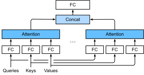
- In practice, it may be beneficial to use different representation subspaces of queries, keys, and values.
Input:
Query vectors: Q
Key vectors: K
Value vectors: V
Output:
\begin{equation} \begin{aligned}\text{MultiHeadAttention}(Q,K,V) & =[\text{head}_{1};\dots;\text{head}_{h}]{\color{red}W^{O}}\\ \text{where head}_{i} & =\text{Attention}(Q{\color{red}W_{i}^{Q}},K{\color{red}W_{i}^{K}},V{\color{red}W_{i}^{V}}),i=1...h \end{aligned} \end{equation} where {\color{red}W_{i}^{Q}},{\color{red}W_{i}^{K}},{\color{red}W_{i}^{V}}, and {\color{red}W^{O}} are parameter matrices to be learned.
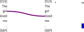
- Multi-head self-attention for the sentence “the girl loved me.” with 12 heads
17.5 Applications
Vision
CNN with Self-Attention
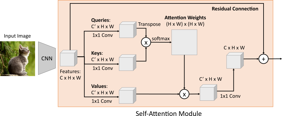
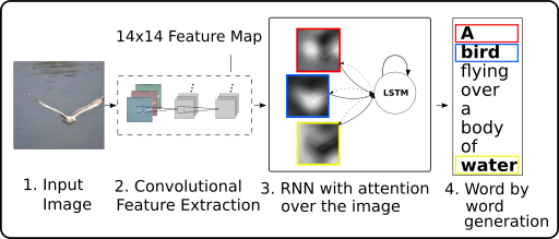
Image Captioning with RNNs and Attention
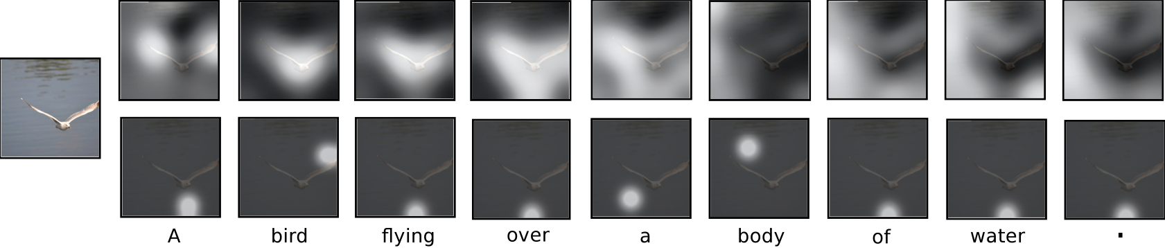
- Attention over time. As the model generates each word, its attention changes to reflect the relevant parts of the image. “soft” (top row) vs “hard” (bottom row) attention.
Transformer
The Transformer
Transformers are a new neural network model that only uses attention!
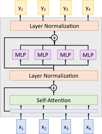
Transformer Block
Input: Set of vectors \boldsymbol{x}
Output: Set of vectors \boldsymbol{y}
Self-attention is the only interaction between vectors!
Layer norm and MLP work independently per vector
Highly scalable, highly parallelizable
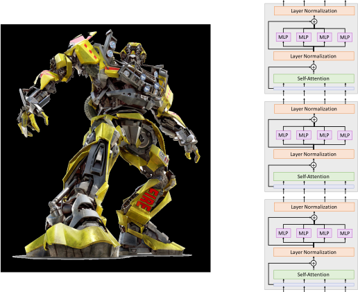
A Transformer is a sequence of transformer blocks
Transfer Learning
“ImageNet Moment for (Natural) Language Processing”
Pretraining:
Download a lot of text from the internet
Train a giant Transformer model for language modeling
Finetuning:
- Fine-tune the Transformer on your own language task
Scaling up Transformers
| Model | Layers | Width | Heads | Params | Data | Training |
|---|---|---|---|---|---|---|
| Transformer-Base | 12 | 512 | 8 | 65M | 8x P100 (12 hours) | |
| Transformer-Large | 12 | 1024 | 16 | 213M | 8x P100 (3.5 days) | |
| BERT-Base | 12 | 768 | 12 | 110M | 13GB | |
| BERT-Large | 24 | 1024 | 16 | 340M | 13GB | |
| XLNet-Large | 24 | 1024 | 16 | ~340M | 126GB | 512x TPU-v3 (2.5 days) |
| RoBERTa | 24 | 1024 | 16 | 355M | 160GB | 1024x V100 GPU (1 day) |
| GPT-2 | 48 | 1600 | ? | 1.5B | 40GB | |
| Megatron-LM | 72 | 3072 | 32 | 8.3B | 174GB | 512x V100 GPU (9 days) |
| Turing-NLG | 78 | 4256 | 28 | 17B | ? | 256x V100 GPU |
| GPT-3 | 96 | 12288 | 96 | 175B | 694GB | ? |