20  MARKOV DECISION PROCESSES

20.1 Markov Processes

Introduction to MDPs

• Markov decision processes formally describe an environment for reinforcement learning

• Where the environment is fully observable

• i.e. The current state completely characterises the process

• Almost all RL problems can be formalised as MDPs, e.g.

  • Optimal control primarily deals with continuous MDPs

  • Partially observable problems can be converted into MDPs

  • Bandits are MDPs with one state

Markov Property

Markov Property

• “The future is independent of the past given the present”

A state S_{t} is Markov if and only if P[S_{t+1}\mid S_{t}]=P[S_{t+1}\mid S_{1},...,S_{t}]

• The state captures all relevant information from the history

• Once the state is known, the history may be thrown away

• i.e. The state is a sufficient statistic of the future

State Transition Matrix

• For a Markov state s and successor state s', the state transition probability is defined by \mathcal{P}_{ss'}=P[S_{t+1}=s'\mid S_{t}=s]

• State transition matrix \mathcal{P} defines transition probabilities from all states s to all successor states s', \begin{array}{cc} & to\\ \mathcal{P}=from & \begin{bmatrix}\mathcal{P}_{11} & \dots & \mathcal{P}_{1n}\\ \vdots\\ \mathcal{P}_{n1} & \dots & \mathcal{P}_{nn} \end{bmatrix} \end{array} where each row of the matrix sums to 1.

Markov Chains

Markov Process

• A Markov process is a memoryless random process, i.e. a sequence of random states S_{1}, S_{2}, … with the Markov property.

A Markov Process (or Markov Chain) is a tuple \left\langle \mathcal{S},\mathcal{P}\right\rangle

• \mathcal{S} is a (finite) set of states

• \mathcal{P} is a state transition probability matrix, \mathcal{P}_{ss'}=\mathcal{P}[S_{t+1}=s'\mid S_{t}=s]

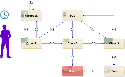
Example: Student Markov Chain

Example: Student Markov Chain Episodes

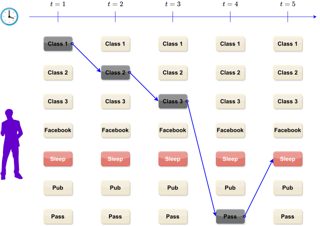
Example: Student Markov Chain Episodes

• Sample episodes for Student Markov Chain starting from S_{1}=C1 S_{1},S_{2},...,S_{T}

• C1 C2 C3 Pass Sleep

• C1 FB FB C1 C2 Sleep

• C1 C2 C3 Pub C2 C3 Pass Sleep

• C1 FB FB C1 C2 C3 Pub C1 FB FB FB C1 C2 C3 Pub C2 Sleep

Example: Student Markov Chain Transition Matrix

		C1	C2	C3	Pass	Pub	FB	Sleep
	C1	0	0.5	0	0	0	0.5	0
	C2	0	0	0.8	0	0	0	0.2
	C3	0	0	0	0.6	0.4	0	0
\mathcal{P}=	Pass	0	0	0	0	0	0	1.0
	Pub	0.2	0.4	0.4	0	0	0	0
	FB	0.1	0	0	0	0	0.9	0
	Sleep	0	0	0	0	0	0	1.0

20.2 Markov Reward Processes

MRP

Markov Reward Process

• A Markov reward process is a Markov chain with values.

A Markov Reward Process is a tuple \left\langle \mathcal{S},\mathcal{P},\mathcal{R},\gamma\right\rangle

• \mathcal{S} is a finite set of states

• \mathcal{P} is a state transition probability matrix, P_{ss'}=P[S_{t+1}=s'\mid S_{t}=s]

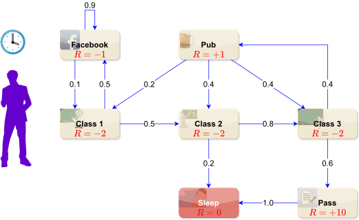
• \mathcal{R} is a reward function, R_{s}=E[R_{t+1}\mid S_{t}=s]

• \gamma is a discount factor, \gamma\in[0,1]

Example: Student MRP

Return

Return

The return G_{t} is the total discounted reward from time-step t. G_{t}=R_{t+1}+\gamma R_{t+2}+\dots=\sum_{k=0}^{\infty}\gamma^{k}R_{t+k+1}

• The discount \gamma\in[0,1] is the present value of future rewards

• The value of receiving reward R after k+1 time-steps is \gamma^{k}R.

• This values immediate reward above delayed reward.

  • \gamma close to 0 leads to ”myopic” evaluation

  • \gamma close to 1 leads to ”far-sighted” evaluation

Why discount?

Most Markov reward and decision processes are discounted. Why?

• Mathematically convenient to discount rewards

• Avoids infinite returns in cyclic Markov processes

• Uncertainty about the future may not be fully represented

• If the reward is financial, immediate rewards may earn more interest than delayed rewards

• Animal/human behaviour shows preference for immediate reward

• It is sometimes possible to use undiscounted Markov reward processes (i.e.\gamma=1), e.g. if all sequences terminate.

Value Function

Value Function

• The value function v(s) gives the long-term value of state s

The state value function v(s) of an MRP is the expected return starting from state s v(s)=E[G_{t}\mid S_{t}=s]

Example: Student MRP Returns

• Sample returns for Student MRP:

• Starting from S_{1}=C1 with \gamma=1 G_{1}=R_{2}+\gamma R_{3}+...+\gamma^{T-2}R_{T}

C1 C2 C3 Pass Sleep	v_{1}=-2-2*\frac{1}{2}-2*\frac{1}{4}+10*\frac{1}{8}	=-2.25
C1 FB FB C1 C2 Sleep	v_{1}=-2-1*\frac{1}{2}-1*\frac{1}{4}-2*\frac{1}{8}-2*\frac{1}{8}	=-3.125
C1 C2 C3 Pub C2 C3 Pass Sleep	v_{1}=-2-2*\frac{1}{2}-2*\frac{1}{4}+1*\frac{1}{8}-2*\frac{1}{8}\dots	=-3.41
C1 FB FB C1 C2 C3 Pub C1 FB FB FB C1 C2 C3 Pub C2 Sleep	v_{1}=-2-1*\frac{1}{2}-1*\frac{1}{4}-2*\frac{1}{8}-2*\frac{1}{8}\dots	=-3.20

Example: State-Value Function for Student MRP

Bellman Equation

Bellman Equation for MRPs

The value function can be decomposed into two parts:

• immediate reward R_{t+1}

• discounted value of successor state \gamma v(S_{t+1})

\begin{align*} v(s) & =E[G_{t}\mid S_{t}=s]\\ & =E[R_{t+1}+\gamma R_{t+2}+\gamma^{2}R_{t+3}+\dots\mid S_{t}=s]\\ & =E[R_{t+1}+\gamma(R_{t+2}+\gamma R_{t+3}+\dots)\mid S_{t}=s]\\ & =E[R_{t+1}+\gamma G_{t+1}\mid S_{t}=s]\\ & =E[R_{t+1}+\gamma v(S_{t+1})\mid S_{t}=s] \end{align*}

v(s)=E[R_{t+1}+\gamma v(S_{t+1})\mid S_{t}=s] v(s)=\mathcal{R}_{s}+\gamma\sum_{s'\in\mathcal{S}}\mathcal{P}_{ss'}v(s')

Example: Bellman Equation for Student MRP

Bellman Equation in Matrix Form

• The Bellman equation can be expressed concisely using matrices, v=\mathcal{R}+\gamma\mathcal{P}v where v is a column vector with one entry per state \begin{bmatrix}v(1)\\ \vdots\\ v(n) \end{bmatrix}=\begin{bmatrix}\mathcal{R}_{1}\\ \vdots\\ \mathcal{R}_{n} \end{bmatrix}+\gamma\begin{bmatrix}\mathcal{P}_{11} & \dots & \mathcal{P}_{1n}\\ \vdots\\ \mathcal{P}_{n1} & \dots & \mathcal{P}_{nn} \end{bmatrix}\begin{bmatrix}v(1)\\ \vdots\\ v(n) \end{bmatrix}

Solving the Bellman Equation

• The Bellman equation is a linear equation

• It can be solved directly: \begin{align*} v & =\mathcal{R}+\gamma\mathcal{P}v\\ (I-\gamma\mathcal{P})v & =\mathcal{R}\\ v & =(I-\gamma\mathcal{P})^{-1}\mathcal{R} \end{align*}

• Computational complexity is O(n^{3}) for n states

• Direct solution only possible for small MRPs

• There are many iterative methods for large MRPs, e.g.

  • Dynamic programming

  • Monte-Carlo evaluation

  • Temporal-Difference learning

20.3 Markov Decision Processes

MDP

Markov Decision Process

• A Markov decision process (MDP) is a Markov reward process with decisions. It is an environment in which all states are Markov.

A Markov Decision Process is a tuple \left\langle \mathcal{S},\mathcal{A},\mathcal{P},\mathcal{R},\gamma\right\rangle

• \mathcal{S} is a finite set of states

• \mathcal{A} is a finite set of actions

• \mathcal{P} is a state transition probability matrix, P_{ss'}^{a}=P[S_{t+1}=s'\mid S_{t}=s,A_{t}=a]

• \mathcal{R} is a reward function, R_{s}^{a}=E[R_{t+1}\mid S_{t}=s,A_{t}=a]

• \gamma is a discount factor, \gamma\in[0,1]

Example: Student MDP

Policies

Policies

A policy \pi is a distribution over actions given states, \pi(a\mid s)=P[A_{t}=a\mid S_{t}=s]

• A policy fully defines the behaviour of an agent

• MDP policies depend on the current state (not the history)

• i.e. Policies are stationary (time-independent), A_{t}\sim\pi(\cdot\mid S_{t}),\forall t>0

• Given an MDP \left\langle \mathcal{S},\mathcal{A},\mathcal{P},\mathcal{R},\gamma\right\rangle and a policy \pi

• The state sequence S_{1}, S_{2}, … is a Markov process \left\langle \mathcal{S},\mathcal{P}^{\pi}\right\rangle

• The state and reward sequence S_{1}, R_{2}, S_{2}, … is a Markov reward process \left\langle \mathcal{S},\mathcal{P}^{\pi},\mathcal{R}^{\pi},\gamma\right\rangle where \begin{align*} \mathcal{P}_{ss'}^{\pi} & =\sum_{a\in\mathcal{A}}\pi(a\mid s)\mathcal{P}_{ss'}^{a}\\ \mathcal{R}_{s}^{\pi} & =\sum_{a\in\mathcal{A}}\pi(a\mid s)\mathcal{R}_{s}^{a} \end{align*}

Value Functions

Value Function

The state-value function v_{\pi}(s) of an MDP is the expected return starting from state s, and then following policy \pi v_{\pi}(s)=\mathbb{E}_{\pi}[G_{t}\mid S_{t}=s]

The action-value function q_{\pi}(s,a) is the expected return starting from state s, taking action a, and then following policy \pi q_{\pi}(s,a)=\mathbb{E}_{\pi}[G_{t}\mid S_{t}=s,A_{t}=a]

Example: State-Value Function for Student MDP

• TO-DO

Bellman Expectation Equation

Bellman Expectation Equation

• The state-value function can again be decomposed into immediate reward plus discounted value of successor state, v_{\pi}(s)=\mathbb{E}_{\pi}[R_{t+1}+\gamma v_{\pi}(S_{t+1})\mid S_{t}=s]

• The action-value function can similarly be decomposed, q_{\pi}(s,a)=\mathbb{E}_{\pi}[R_{t+1}+\gamma q_{\pi}(S_{t+1},A_{t+1})\mid S_{t}=s,A_{t}=a]

Bellman Expectation Equation for v_{\pi}

v_{\pi}(s)=\sum_{a\in\mathcal{A}}\pi(a\mid s)q_{\pi}(s,a)

Bellman Expectation Equation for q_{\pi}

q_{\pi}(s,a)=\mathcal{R}_{s}^{a}+\gamma\sum_{s'\in\mathcal{S}}\mathcal{P}_{ss'}^{a}v_{\pi}(s')

v_{\pi}(s)=\sum_{a\in\mathcal{A}}\pi(a\mid s)\left(\mathcal{R}_{s}^{a}+\gamma\sum_{s'\in\mathcal{S}}\mathcal{P}_{ss'}^{a}v_{\pi}(s')\right)

q_{\pi}(s,a)=\mathcal{R}_{s}^{a}+\gamma\sum_{s'\in\mathcal{S}}\mathcal{P}_{ss'}^{a}\sum_{a'\in\mathcal{A}}\pi(a'\mid s')q_{\pi}(s',a')

Example: Bellman Expectation Equation in Student MDP

Bellman Expectation Equation (Matrix Form)

• The Bellman expectation equation can be expressed concisely using the induced MRP, v_{\pi}=\mathcal{R}^{\pi}+\gamma\mathcal{P}^{\pi}v_{\pi} with direct solution v_{\pi}=(I-\gamma\mathcal{P}^{\pi})^{-1}\mathcal{R}^{\pi}

Optimal Value Function

Optimal Value Function

The optimal state-value function v_{*}(s) is the maximum value function over all policies v_{*}(s)=\max_{\pi}v_{\pi}(s) The optimal action-value function q_{*}(s,a) is the maximum action-value function over all policies q_{*}(s,a)=\max_{\pi}q_{\pi}(s,a)

• The optimal value function specifies the best possible performance in the MDP.

• An MDP is “solved” when we know the optimal value fn.

Example: Optimal Value Function for Student MDP

• TO-DO

Example: Optimal Action-Value Function for Student MDP

• TO-DO

Optimal Policy

• Define a partial ordering over policies \pi\geq\pi'\text{ if }v_{\pi}(s)\geq v_{\pi'}(s),\forall s

For any Markov Decision Process

• There exists an optimal policy \pi_{*} that is better than or equal to all other policies, \pi_{*}\geq\pi,\forall\pi

• All optimal policies achieve the optimal value function, v_{\pi_{*}}(s)=v_{*}(s)

• All optimal policies achieve the optimal action-value function, q_{\pi_{*}}(s,a)=q_{*}(s,a)

Finding an Optimal Policy

• An optimal policy can be found by maximising over q_{*}(s,a) \pi_{*}(a\mid s)=\begin{cases} 1 & \text{if }a=\arg\max_{a\in\mathcal{A}}q_{*}(s,a)\\ 0 & \text{otherwise} \end{cases}

• There is always a deterministic optimal policy for any MDP

• If we know q_{*}(s,a), we immediately have the optimal policy

Example: Optimal Policy for Student MDP

• TO-DO

Bellman Optimality Equation for v_{*}

• The optimal value functions are recursively related by the Bellman optimality equations: v_{*}(s)=\max_{a}q_{*}(s,a)

Bellman Optimality Equation for q_{*}

q_{*}(s,a)=\mathcal{R}_{s}^{a}+\gamma\sum_{s'\in\mathcal{S}}\mathcal{P}_{ss'}^{a}v_{*}(s')

v_{*}(s)=\max_{a}\mathcal{R}_{s}^{a}+\gamma\sum_{s'\in\mathcal{S}}\mathcal{P}_{ss'}^{a}v_{*}(s')

q_{*}(s,a)=\mathcal{R}_{s}^{a}+\gamma\sum_{s'\in\mathcal{S}}\mathcal{P}_{ss'}^{a}\max_{a'}q_{*}(s',a')

Example: Bellman Optimality Equation in Student MDP

Solving the Bellman Optimality Equation

• Bellman Optimality Equation is non-linear

• No closed form solution (in general)

• Many iterative solution methods

  • Value Iteration

  • Policy Iteration

  • Q-learning

  • Sarsa

20.4 Extensions to MDPs

Extensions to MDPs

• Infinite and continuous MDPs

• Partially observable MDPs

• Undiscounted, average reward MDPs

Infinite MDPs

Infinite MDPs

The following extensions are all possible:

• Countably infinite state and/or action spaces

  • Straightforward

• Continuous state and/or action spaces

  • Closed form for linear quadratic model (LQR)

• Continuous time

  • Requires partial differential equations

  • Hamilton-Jacobi-Bellman (HJB) equation

  • Limiting case of Bellman equation as time-step \to 0

Partially Observable MDPs

POMDPs

A Partially Observable Markov Decision Process is an MDP with hidden states. It is a hidden Markov model with actions.

A POMDP is a tuple \left\langle \mathcal{S},\mathcal{A},\mathcal{O},\mathcal{P},\mathcal{R},\mathcal{Z},\gamma\right\rangle

• \mathcal{S} is a finite set of states

• \mathcal{A} is a finite set of actions

• \mathcal{O} is a finite set of observations

• \mathcal{P} is a state transition probability matrix, P_{ss'}^{a}=P[S_{t+1}=s'\mid S_{t}=s,A_{t}=a]

• \mathcal{R} is a reward function, R_{s}^{a}=\mathbb{E}[R_{t+1}\mid S_{t}=s,A_{t}=a]

• \mathcal{Z} is an observation function, Z_{s'o}^{a}=P[O_{t+1}=o\mid S_{t+1}=s',A_{t}=a]

• \gamma is a discount factor, \gamma\in[0,1]

Belief States

A history H_{t} is a sequence of actions, observations and rewards, H_{t}=A_{0},O_{1},R_{1},...,A_{t-1},O_{t},R_{t}

A belief state b(h) is a probability distribution over states, conditioned on the history h b(h)=(P[S_{t}=s_{1}\mid H_{t}=h],...,P[S_{t}=s_{n}\mid H_{t}=h])

Reductions of POMDPs

• The history H_{t} satisfies the Markov property

• The belief state b(H_{t}) satisfies the Markov property

• A POMDP can be reduced to an (infinite) history tree

• A POMDP can be reduced to an (infinite) belief state tree

Average Reward MDPs

Ergodic Markov Process

An ergodic Markov process is

• Recurrent: each state is visited an infinite number of times

• Aperiodic: each state is visited without any systematic period

An ergodic Markov process has a limiting stationary distribution d_{\pi}(s) with the property d_{\pi}(s)=\sum_{s'\in\mathcal{S}}d_{\pi}(s')P_{s's}

Ergodic MDP

An MDP is ergodic if the Markov chain induced by any policy is ergodic.

• For any policy \pi, an ergodic MDP has an average reward per time-step \rho_{\pi} that is independent of start state. \rho_{\pi}=\lim_{T\to\infty}\frac{1}{T}\mathbb{E}\left[\sum_{t=1}^{T}R_{t}\right]

Average Reward Value Function

• The value function of an undiscounted, ergodic MDP can be expressed in terms of average reward.

• \tilde{v}_{\pi}(s) is the extra reward due to starting from state s, \tilde{v}_{\pi}(s)=\mathbb{E}_{\pi}\left[\sum_{k=1}^{\infty}(R_{t+k}-\rho_{\pi})\mid S_{t}=s\right]

• There is a corresponding average reward Bellman equation, \begin{align*} \tilde{v}_{\pi}(s) & =\mathbb{E}_{\pi}\left[(R_{t+1}-\rho_{\pi})+\sum_{k=1}^{\infty}(R_{t+k+1}-\rho_{\pi})\mid S_{t}=s\right]\\ & =\mathbb{E}_{\pi}\left[(R_{t+1}-\rho_{\pi})+\tilde{v}_{\pi}(S_{t+1})\mid S_{t}=s\right] \end{align*}

20.5 References

• Youtube: Markov Decision Processes